Modern datacenters are susceptible to various types of failures in the field, such as fail-stop, fail-partial, and Byzantine. The recent advancement in both software and hardware pushes the previously overlooked fail-slow failure to the fore. Fail-slow components, stuck in an intermediate state between full-speed and non-functional, tend to exhibit rather low performance. Prior work and our analysis suggest that fail-slow failures are not only prevalent but also impactful in the field. In this article, we share our lessons and experiences in building a practical fail-slow detection framework for storage devices in the cloud.
Fail-Slow in the Wild
Severity
The fail-slow failure is a widespread and severe issue for the datacenters. First, recent studies on storage systems reliability have shown that the annual fail-slow rate, ranging from 1% to 2%, is already as frequent as annual fail-stop incidents [7, 9]. Second, fail-slow failures, especially the transient ones, can often be ignored or misinterpreted as performance variations. In this case, it is hard for on-site engineers to pinpoint fail-slow, much less reproduce or reason the root causes [3]. Most importantly, fail-slow failures can have a significant impact on the I/O performance in the wild.
Hard to Detect
Accurate detection of fail-slow failures is challenging. Normal performance variations (e.g., triggered by workload burst or SSD internal garbage collection) may generate symptoms similar to fail-slow failures. In contrast to fail-stop failures where the criterion is well-defined (i.e., working or stopped working), there are a thousand ways to define fail-slow. On-site engineers, for example, are frequently perplexed and wonder how slow a component must be to be labeled fail-slow. When there are no golden standards, the detection procedure would be empirical and hence necessarily inaccurate.
Existing solutions to fail-slow detection in storage systems are impractical and inefficient for large-scale cloud deployment. First, these solutions require source code access or software modification (e.g., modifying software timeouts in IASO [9]), whereas cloud vendors like us do not touch tenants’ code. Even for in-house storage infrastructures, inserting certain code segments is still time-consuming since the systems might operate dozens of internal services with varying software stacks. Second, existing solutions can only identify fail-slow failures at the node level (e.g., IASO), thus still requiring nontrivial manual efforts to locate the culprits.
Design Goals of Fail-slow Detection
From our perspective, a practical fail-slow detection framework should have the following properties.
- Non-intrusive. We as cloud service providers cannot alter users’ software or require them to run certain modified versions of software stacks. Instead, we may only make use of external performance statistics like drive latency to detect fail-slow.
- Fine-grained. Fail-slow root cause diagnosis can often be time-consuming (from days to even weeks [3, 9]). The framework is expected to directly pinpoint the culprit.
- Accurate. The framework should have satisfying precision and recall to avoid unnecessary diagnosis of false positives.
- General. The framework can be quickly applied to different cloud services (like block storage and database) with minor adjustments.
Alibaba Storage System Architecture
Our data centers follow a classic distributed storage system setup. We have multiple Internet Data Centers (IDCs) across the world. Each IDC includes multiple storage clusters. Atop each cluster, a distributed file system (DFS) is deployed to support a dedicated service (e.g., block storage, NoSQL, or big data analysis). Each cluster consists of tens of racks (at most 200), and each rack contains dozens of nodes (at most 48). Each node contains dozens of storage devices (HDDs or SSDs) that are by default from the same drive model. A more detailed description of our architecture can be found in our paper [6] and open dataset [1].
Dataset Description
In our data centers, a monitoring daemon is placed in each node to collect operational statistics, mainly the latency and throughput of each drive. The daemons calculate the average statistics every 15 seconds and record them as time-series data entries. The daemons run three hours a day (from 9PM to 12AM). A drive generates 720 entries (= 180 min×4 entries/min) per day. In total, we have compiled around 100 billion entries as our dataset.
We have explored multiple solutions to fail-slow detection at Alibaba. In this section, we discuss three unsuccessful attempts over the years and summarize these early efforts into a series of lessons learned as design guidelines of PERSEUS.
Attempt 1: Threshold Filtering
Methodology. Intuitively, we can set up a hard threshold on drive latency to identify fail-slow drives based on the Service Level Objectives (SLOs). To avoid mislabeling due to one-off events such as SSD internal Garbage Collection (GC), we further specify a minimum slowdown span for a suspicious drive to be considered fail-slow.
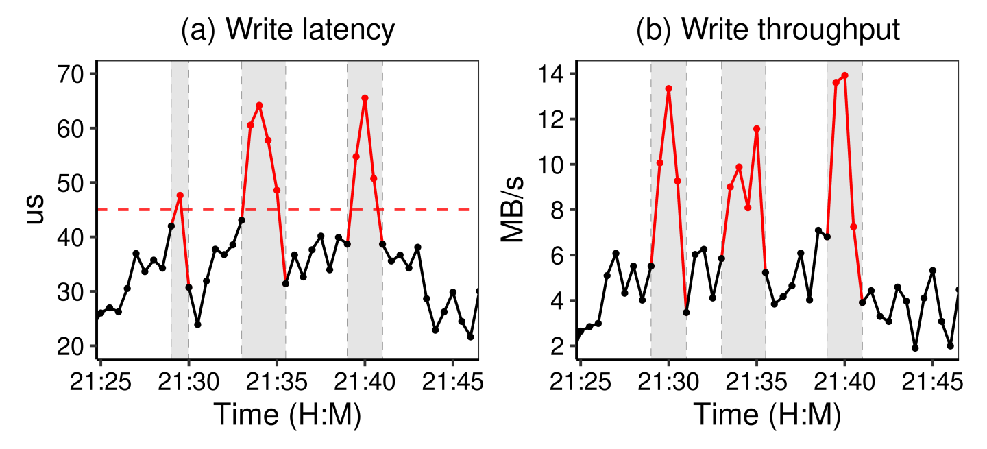
Limitation. The detection accuracy of threshold filtering is low, as the latency is highly influenced by the workloads. Here, we use the latency and throughput traces of an NVMe SSD from the block storage service as an example. The left of Figure 1 illustrates the latency variation of the drive where the horizontal dashed line indicates the threshold (45µs). The right of Figure 1 is the corresponding throughput. We can see that three latency spikes occur at around 21:29, 21:34, and 21:40 as the latency increases to 65µs. By comparing latency with throughput, it is clear that the workload pressure causes these spikes.
Hence, the dilemma is as follows. Setting a relaxed threshold easily mislabels normal performance variations as fail-slow events. Meanwhile, a strict one could leave many fail-slow cases undiscovered. Further, using a set of thresholds for different scenarios through fine-tuning can be fairly time-consuming as our experiments show that latency variation is a factor of drive models and workloads. In practice, we use threshold-based detection as a fail-safe measure like timeouts.
Attempt 2: Peer Evaluation
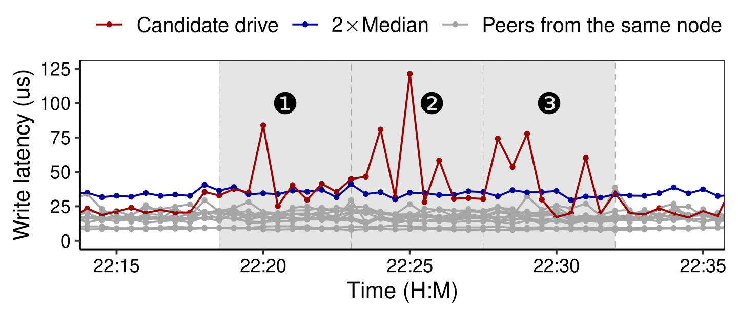
Methodology. The problem with the first attempt is not having an adaptive threshold for detection. To address this problem, we explored the idea of peer evaluation [4, 7]. The rationale behind this approach is that, with load balancing across the distributed storage system, drives from the same node should receive similar workload pressure. Since fail-slow failures are relatively rare [3] and the majority of drives in a node should be normal, we can identify the fail-slow drive by comparing the performance between drives from the same node.
Specifically, we first calculate the node-level moving median latency for every 15 seconds. We then evaluate whether there are drives constantly (more than half of the time) delivering abnormal performance—twice slower than the median in our case—during the monitoring window (e.g., 5 minutes). If so, the detection framework reports a fail-slow event, and the monitoring window moves forward to start the next round of evaluation.
Attempt 3: IASO-Based Model
Methodology. IASO is a fail-slow detection framework focusing on identifying performance-degrading nodes [9]). The design principle of IASO is to leverage software timeouts and convert them into informative metrics to benchmark fail-slow. However, directly using IASO is not suitable for us. First, IASO requires code changes (i.e., intrusive monitoring) to insert or modify certain code snippets of the running instances (e.g., Cassandra and ZooKeeper), thus leveraging software-level timeouts to identify fail-slow incidents. Second, IASO is node-level detection, whereas our goal is device-level. Nevertheless, we re-factor IASO with our best effort. To avoid modifying the software, we reuse the fail-slow event reporting by peer evaluation from Attempt 2.
Limitation. The IASO-based model delivers rather unsatisfactory performance on our assembled benchmark, with a precision rate of only 0.48. We suspect the main reason is that using the fail-slow event reporting to replace the software timeout might not be effective. Moreover, we have explored other possible alternatives, such as replacing software timeouts with thresholds. However, the results are still unsatisfactory. Therefore, we believe IASO may not achieve our goals even with refactoring.
Guidelines for PERSEUS
Requirement 2: How to automatically derive adaptive thresholds?
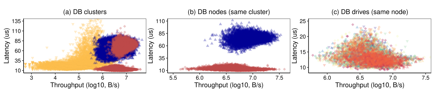
Although peer evaluation in Attempt 2 can provide adaptive thresholds, it requires time-consuming tuning for different service types and drive models. Now, with workload pressure modeled by throughput, we are able to build the latency-vs-throughput (LvT) distribution. Then, we can use regression models on such distribution to define a statistically normal drive and subsequently use its upper bound as the adaptive threshold for various environments.
To build such regression models, we need to determine the scope of drives to be included in the LvT distribution. The tradeoff is that including more samples (e.g., all drives from the service) can be more statistically confident but subject to a more diverse distribution—difficult to derive a clear upper bound. Therefore, we plot the distribution at three different scales in Figure 3 and discuss their pros and cons as follows.
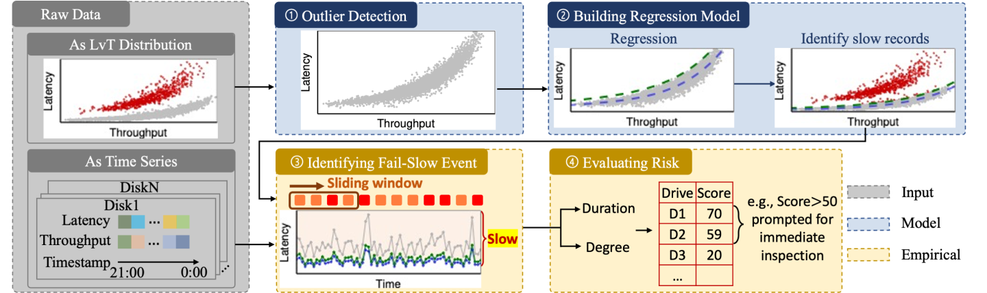
With lessons from previous attempts, we propose PERSEUS, a non-intrusive, fine-grained and general fail-slow detection framework. As illustrated in Figure 4, the core idea of PERSEUS is building a polynomial regression on the node-level LvT distribution to automatically derive an adaptive threshold for each node. PERSEUS can use the threshold to formulate fail-slow events and further use a scoreboard mechanism to single out the drives with severe fail-slow failures. In this section, we discuss the design of each step at length.
Step 1: Outlier Detection
Before applying regression models, a necessary pre-process is to root out noisy samples (i.e., outliers). While the LvT samples (i.e., <latency, throughput> pairs) are usually clustered together within a node, entries from fail-slow drives or under normal performance variations (e.g., internal GC) can still be deviating. Therefore, before building a polynomial regression model, we first screen out the outliers.
Using DBSCAN. Density-based clustering algorithms (measuring the spatial distance) are promising approaches for identifying the potentially distinctive groups (i.e., normal vs. slow). Initially, we employ DBSCAN [10] to label outliers. In a nutshell, DBSCAN groups points that are spatially close enough—distances between points are smaller than a minimum value. Note that <latency, throughput> pairs from long-term or permanent fail-slow drives can be clustered together but far away from the main cluster. Hence, we only keep one group with the most points for further modeling.
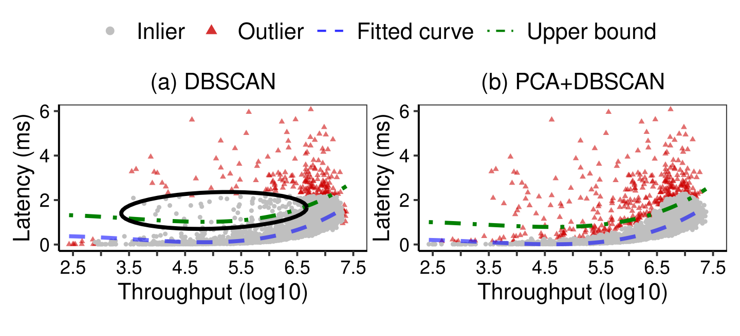
Adding PCA. Using DBSCAN alone can have limited effectiveness. Here, we choose a sample node with one confirmed fail-slow drive to illustrate the limitation. In Figure 5a, we apply fine-tuned DBSCAN (outliers in red points) to the node’s daily raw dataset and fit the rest of the data (grey points) to polynomial regression (with a fitted curve in blue and a 99.9% prediction upper bound in green dashed line). In this example, the DBSCAN algorithm only identifies 63.83% of slow entries.
The root cause is that the throughput and latency are positively correlated. Thus, the samples (i.e., <latency, throughput> pairs) can be skewed towards a particular direction. Hence, outliers (i.e., samples from fail-slow drives) can be mislabeled as inliers (see the black circle in Figure 5a). Therefore, we leverage Principal Component Analysis (PCA [2]) to transform the coordinates and penalize the outliers perpendicular to the skewed direction in order to reduce mislabeling. As a result, applying DBSCAN with PCA effectively detects 92.55% of slow entries (see Figure 5b).
Usage of outliers. In RQ3, we have discussed that just using binary detection cannot reflect the extent of slowdown. Therefore, we do not directly use the binary results of outlier detection, such as simply labeling outliers as slow entries (i.e., skipping Step 2) or fail-slow events (i.e., skipping Step 2 and Step 3). Rather, we exclude the outliers to build a better-fitted model for measuring the slowdown degree of entries.
Step 2: Regression Model
Step 3: Identifying Fail-Slow Event
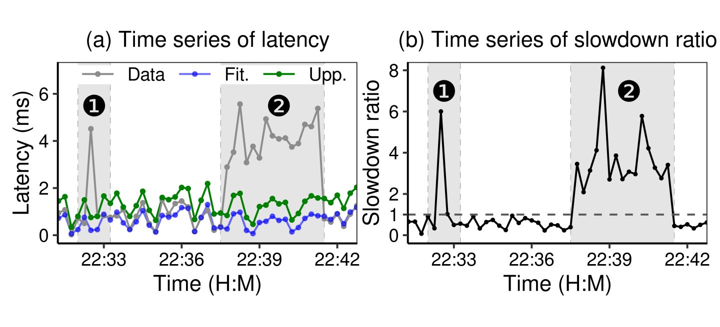
Formulating events. First, we calculate a time series of Slowdown Ratio (SR), which is obtained by dividing drive latency by the prediction upper bound entry by entry (every 15 seconds). We then formulate fail-slow events by using a sliding window (similar to Attempt 2). The sliding window has a fixed length (i.e., a minimum span) and starts at the first entry. Within the span, if a certain proportion of SR series has a median SR value exceeding a threshold, PERSEUS would record that the drive has encountered a fail-slow event within the span and see if the event should be extended to the next entry. In practice, we only formulate fail-slow events under a persistent series of slowdown entries as one-off spike entries are likely to be acceptable performance variations. In Figure 6b, while both (1) and (2) have high SR values, only (2) would be marked as a fail-slow event.
Step 4: Risk Score
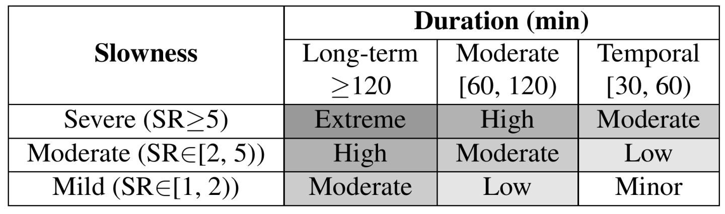
Therefore, we adopt the idea of establishing a risk score mechanism from performance regression testing [5] to quantify the severity of fail-slow. First, slowdown duration and severity are classified into different risk levels as illustrated in Table 1. For example, extreme risk of fail-slow corresponds to drives with a long-term daily slowdown span (over 120 minutes) and severe slowness (SR≥5). Furthermore, a per-drive risk score is calculated by assigning different weights to risk levels:
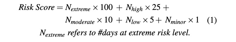
If a drive whose risk scores exceed a minimum value within a few days, the drive will be recommended for immediate isolation and hardware inspection. Note that all drives in our fleet, HDDs and SSDs, use the same scoring mechanism.
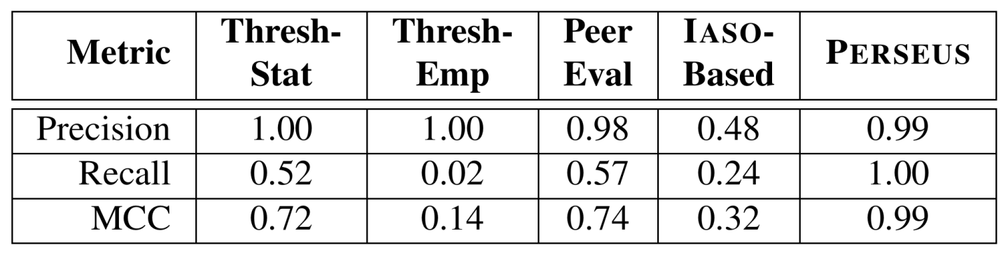
We have assembled the first large-scale, clear-labeled public dataset on real-world operational traces aiming at fail-slow detection. The dataset has been released to the public for fail-slow study [1]. Based on this dataset, we extensively evaluate previous attempts and PERSEUS. We adopt three evaluation metrics: precision rate, recall rate, and Matthews Correlation Coefficient (MCC [8]). Table 2 summarizes the performance results. Clearly, PERSEUS outperforms all previous attempts. The high precision and recall indicate that PERSEUS can successfully detect all fail-slow drives while rarely mislabeling normal as fail-slow. Therefore, we conclude that PERSEUS achieves our design goals as a fine-grained (per-drive), non-intrusive (no code changes), general (same set of parameters for different setups) and accurate (high precision and recall) fail-slow detection framework.
In this paper, we first share our unsuccessful attempts in developing robust and non-intrusive fail-slow detection for large-scale storage systems. We then introduce the design of PERSEUS, which utilizes classic machine learning techniques and scoring mechanisms to achieve effective fail-slow detection. Since deployment, PERSEUS has covered around 250K drives and successfully identified 304 fail-slow drives. We have released our dataset as an open benchmark dedicated to fail-slow drive detection.