
We also observe that Binsearch, Binsearch with Seeding, and Linear with Seeding are robust across the workloads, but the model-guided policy is unstable. This is not surprising given that the accuracy of the learned model guides the search. As Section 3.6 explains, if the model is inaccurate the search may converge slowly.
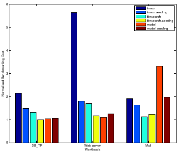
The linear policy is inefficient and highly sensitive to the magnitude of peak
rate. The benchmarking cost of Linear for Web server peaks at a
higher absolute value for all samples than for DB_TP and Mail,
causing more than a factor of ![]() increase in the total cost for mapping the
surface. Note that for Mail, Binsearch with Seeding incurs a
slightly higher cost than Binsearch. For some configurations, as
Section 3.7 explains, seeding can incur additional cost to recover
from a bad seed resulting in longer search times.
increase in the total cost for mapping the
surface. Note that for Mail, Binsearch with Seeding incurs a
slightly higher cost than Binsearch. For some configurations, as
Section 3.7 explains, seeding can incur additional cost to recover
from a bad seed resulting in longer search times.
 |
Reducing the Number of Samples. To evaluate the RSM approach presented in
Section 4, we approximate the response surface by a
quadratic curve in two dimensions: peak rate = func(number of disks, number of
nfsds). We use a D-optimal design [17] from RSM to obtain the best
of ![]() ,
, ![]() and
and ![]() samples out of a total of
samples out of a total of ![]() samples for learning the
response surface equation. We use Binsearch to obtain the
peak rate for each.
samples for learning the
response surface equation. We use Binsearch to obtain the
peak rate for each.
After learning the equation, we use it to predict the peak rate at all the other samples in the surface. Table 4 presents the mean absolute percentage error in predicting the peak rate across all the samples. The results show that D-optimal designs do a very good job of picking appropriate samples, and that very little more can be learned by small increases in the number of points sampled. Improving the accuracy of the surface with limited numbers of sampled points is an area of ongoing research.
|
varun 2008-05-13