
The aggregate performance improvement from the passive
measurement-based schemes is shown in Figure 6. Here,
we set the EWMA parameter ![]() so that only the current
measurement samples are used to estimate provider performance, and
select a sampling interval of 30s. The figure plots the performance
for the five client workloads. In addition, we show the performance
from using the three providers individually.
so that only the current
measurement samples are used to estimate provider performance, and
select a sampling interval of 30s. The figure plots the performance
for the five client workloads. In addition, we show the performance
from using the three providers individually.
The performance improvement relative to the best individual provider is significant - about 20-25% for the heavy workloads (right end of the graph) and about 10-15% for the light workloads (left end of the graph). The performance is still about 15-20% away from the optimal value of 1, however. The results for other sampling intervals (60s, 120s, 300s and 450s) are similar, and are omitted for brevity. The performance improvements from using the active measurement-based schemes are also similar and are discussed later.
Figures 7(a) and (b) illustrate the distribution of the
response time improvements offered by the passive measurement scheme
(for ![]() and sampling interval = 30s) relative to being
singly-home to the best provider from Figure 6, i.e.,
ISP 3. Figure (a) plots the CDF of the ratio of the response time from
using ISP 3 to the response time from the passive measurement scheme
across all transfers. These results are for the specific instance
where the client arrival rate is 13.3 requests/s at the server. Figure
(b) similarly plots the difference in the response times for the
same client workload.
and sampling interval = 30s) relative to being
singly-home to the best provider from Figure 6, i.e.,
ISP 3. Figure (a) plots the CDF of the ratio of the response time from
using ISP 3 to the response time from the passive measurement scheme
across all transfers. These results are for the specific instance
where the client arrival rate is 13.3 requests/s at the server. Figure
(b) similarly plots the difference in the response times for the
same client workload.
Notice, from either figure, that the passive measurement scheme improves the response time performance for over 65% of the transfers. Figure 7(a) shows that this route control scheme improves the response times by factors as large as 5 for a small fraction of transfers (about 1%), relative to being singly-homed. Similarly, Figure 7(b) shows that the scheme can improve the response time by more than 1s for some transfers. Notice also, from either figure, that the passive measurement-based scheme ends up offering sub-optimal performance for about 35% of the transfers.
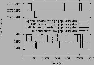 |
Figure 8 illustrates the operation of the passive measurement-based scheme. In this figure, we show the providers used over time for transfers to three different destinations - a popular destination (10.1.1.4), a moderately popular destination (10.1.1.16), and a less popular destination (10.1.1.38). Recall that the passive measurement-based scheme explicitly tracks and controls candidate paths to the 40 most popular destinations. The sampling interval is 30s and the client arrival rate is about 13.3 requests/s.
From this figure, we see that changes to the route for the popular destination is made every 160s on an average. For the moderate and less popular destinations, the intervals are 300s and 550s respectively. For the passive scheme, the number of route changes depends on the popularity of the destinations - the more popular a destination is, the higher the frequency of its route changes. Figure 8 also shows the optimal choice of providers for the popular destination as a function of time, as determined from the underlying delay traces. Comparing this with the ISPs actually selected by the scheme for this destination illustrates cases where the scheme sometimes makes a sub-optimal choice (e.g., between 750-800s, around 1500s, and 2250-2450s).