|
USENIX 2006 Annual Technical Conference Refereed Paper
[USENIX 2006 Annual Technical Conference Technical Program]
SMART: An Integrated Multi-Action Advisor for Storage Systems
Li Yin
University of California, Berkeley
Sandeep Uttamchandani
IBM Almaden Research Center
Madhukar Korupolu
IBM Almaden Research Center
Kaladhar Voruganti
IBM Almaden Research Center
Randy Katz
University of California, Berkeley
The designers of clustered file systems, storage resource
management software and storage virtualization devices are trying to
provide the necessary planning functionality in their products to facilitate the invocation of the
appropriate corrective actions in order to satisfy user specified service level objectives (SLOs).
However, most existing approaches only perform
planning for a single type of action such as workload throttling, or
data migration, or addition of new resources.
As will be shown in this paper, single action based plans are not always cost effective.
In this paper we present a framework SMART that considers multiple types of corrective
actions in an integrated manner and generates a combined corrective
action schedule. Furthermore, often times, the best cost-effective schedule for a one-week
lookahead could be different from the best cost-effective schedule for a
one-year lookahead. An advantage of the SMART framework is that it considers
this lookahead time window in coming up with its corrective action schedules.
Finally, another key advantage
of this framework is that it has a built-in mechanism to handle unexpected surges in workloads.
We have implemented our framework and algorithm as part of a clustered
file system and performed various experiments to show the benefits of
our approach.
With an increase in the number of applications, the amount of managed storage,
and the number of policies and best practices, system administrators
and designers are finding it extremely difficult to generate cost
effective plans that can satisfy the storage needs of the storage applications.
Typically, system administrators over provision their storage resources
due to lack of proper storage management tools.
Thus, the vendors of file systems, storage resource management software
and storage virtualization boxes are trying to have the ability to
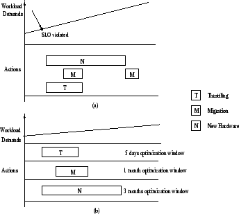
Figure 1:
Planning Issues
 |
automatically
monitor resource utilization and workload SLOs, analyze
the source of the problem, plan a corrective action, and invoke
corrective actions to make the necessary changes.
Research prototypes and products
that perform the above tasks are beginning to appear. However,
these tools suffer from the following two key drawbacks with respect to the
planning aspect of the solution:
Single Action Based: Existing effort has focused on
using a single type of corrective action such as workload
throttling, data migration, or adding more resources to correct
SLO violations. These tools lack the ability to combine the
different types of corrective actions to provide better cost
trade-off points. When the SLO for a workload gets violated
there will be situations where a combination of actions would provide
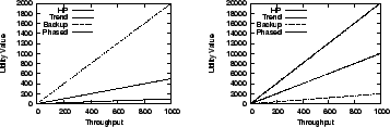
the most optimum cost savings. For example, in Figure 1
(a), upon the violation of the SLO, it is desirable
to throttle the workload until the data associated with the workload
can be migrated to a less contended array rank, and if necessary can
be eventually migrated to a new rank that is part of a newly
provisioned array. Thus, there is a need for a planning tool that can
advise the administrators to take the right action or a combination of
actions at the right time. Currently, the storage management
eco-systems from various vendors provide good domain specific
planning tools such as network planning, storage controller planning,
migration planning etc. However, most of these tools are not
integrated with each other. For example, capacity planning (typically considered a long term action)
is not well integrated with throttling planning (an instantaneous action).
Lack of proper integration between the planning
tools transfers the responsibility of integration
to a system administrator. As discussed above, this
becomes difficult as the system size scales up. Typically this
results in solutions that are either grossly over-provisioned with
excess capacity or under-provisioned to
meet service level agreements (SLOs).
Single time-window based optimization: Another
drawback of existing tools is that they take a
``one-size fits all'' approach to the problem. For example, the solution
(workload throttling) that is the most cost effective for one
week might be different from the solution (adding new
hardware) that is the most optimum for one year. Time is an important
aspect and often overlooked part of the planning process. That is,
cost-wise different solutions could be optimal during different
observation windows. Currently, most storage planning tools do not
allow administrators to evaluate plans for different observation time
windows. This results in the administrators not taking the right
action at the right time. For example, as shown in Figure 1 (b),
different solutions are optimal for different time windows: (1)
If the optimization time window is five days, throttling is the most
optimal solution. (2)
If the optimization time window is one month, data migration is the
most cost effective solution.
(3) If the optimization time window is three months, addition of new
hardware is the most cost effective solution.
In this paper, we propose an action schedule framework called
SMART. The key contributions of SMART are:
Integrated multi-action planning: We provide an action
scheduling algorithm that allows combining seemingly disparate
storage management actions such as workload throttling,
data migration, and resource provisioning into an integrated framework.
Multi-granularity temporal planning: Our
algorithm allows for the specification of optimization time
windows. For example, one could indicate that they want the solution
that is the most cost effective for either one day or one year.
Action selection for unexpected workload variations:
Our core algorithm (contribution number 1) can determine whether the surge in
the I/O requests is an unknown workload spike or a known trend and select
corrective actions accordingly.
Deployment of the framework in a file-system: In order to
validate the benefits described above, we have implemented
our framework and algorithm as part of the GPFS: a scalable shared-disk file system [21].
GPFS performs its own logical volume management.
We have evaluated our implementation and the results are presented in the
experiment section. It is to be noted that the framework
and algorithm are general enough to be deployed as part of
storage resource management and storage
virtualization software.
2 Framework for SMART
Figure 2:
Architecture of Action Scheduler
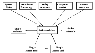 |
This section describes the framework of SMART (shown in Figure
2). SMART can be deployed in file systems,
storage resource management software and storage virtualization boxes
(details of the file system deployment are given in Section 4).
The key components of SMART are:
Input modules: They include sensors monitoring the system state  ,
specifications for administrator-defined business-level constraints (budget constraints
and optimization window), SLOs, utility functions, time-series forecasting of workload request-rate,
and component models for the storage devices. Here, the system state represents the run-time
details of the system and is defined as a triplet ,
specifications for administrator-defined business-level constraints (budget constraints
and optimization window), SLOs, utility functions, time-series forecasting of workload request-rate,
and component models for the storage devices. Here, the system state represents the run-time
details of the system and is defined as a triplet
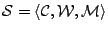 ,
where ,
where  is the set of components in the system, is the set of components in the system,
 is the workloads and is the workloads and  is the current
mapping of workloads to the components. is the current
mapping of workloads to the components.
Utility evaluator: It calculates the overall utility
value in a given system state. It uses component models to
interpolate the IO performance values which in turn map to the utility
delivered to the workloads.
Single action tools: They decide the optimal invocation
parameters for a corrective action in a given system state. SMART can
leverage existing tools for individual corrective actions namely throttling
[25,9,17], migration [10,16],
and provisioning [5,3].
Action Advisor: This is the core of SMART that aims to
improve storage system utility for a given optimization window and
business-level constraints. It interacts with the single action tools
and generates a time-based action schedule with details of what action
to invoke, when to invoke and how to invoke. This is accomplished by
feeding the action tools with different system states and collecting
individual action options. The Action Advisor then analyzes the selected
action invocation parameters using the Utility Evaluator (details of
the algorithm are presented in Section 3). The Action Advisor
can operate both reactively (when SLO has been violated) as well as
proactively (before SLO violation happens).
This section covers the details of the
framework. We will present the details of the algorithm for the Action Advisor
in the next section.
For the input modules described below, there are several different
techniques that are available - the focus of this paper is to demonstrate how
these building blocks work together to solve the
problem, rather than their internal details.
Time-series Forecasting
The forecasting of future workload demands is based on extracting
patterns and trends from historical data. There are several well-known approaches
for time series analysis of historic data such as ARIMA [24] and
Neural Network [8]. The general form of time-series functions is as
follows:
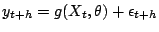 |
(1) |
where:  is the variable(s) vector to be forecast. is the variable(s) vector to be forecast.
 is the time when the forecast is made. is the time when the forecast is made.  are predictor
variables, which usually includes the observed and lagged values of
till time . are predictor
variables, which usually includes the observed and lagged values of
till time .  is the vector of parameter of the
function is the vector of parameter of the
function  and and
 is the prediction error. is the prediction error.
Utility functions
The concept of utility function has been introduced to evaluate
the degree of user's satisfaction.
There are several different techniques to specify utility functions.
For SMART, the utility function associates workloads performance with
a utility value, which reflects the user's degree of satisfaction.
The utility function for each workload can be (1) provided by the administrators; (2) defined in terms of priority value and SLOs; or (3) defined by
associating a dollar value to the level of service delivered, e.g., $1000/GB
if the latency is less than 10ms, otherwise $100/GB.
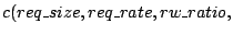
Component models
A component model predicts values of a delivery metric
as a function of
workload characteristics. SMART can in principle accommodate models
for any system component.
In particular, the model for a storage
device takes the form:
Response_time =
Creating component models is an area of active ongoing research.
Models based on simulation or emulation [12,29] require a fairly detailed
knowledge of the system's internals; analytical models [22,19]
require less, but device-specific information must still be taken
into account to obtain accurate predictions.
Black-box [4,26]
models are built by recording and correlating inputs and
outputs to the system in diverse states, without regarding its
internal structure.
Since SMART needs to explore a large candidate
space in a short time, simulation based approaches are not feasible due
to the long prediction overhead. Analytical models and
black box approaches both work with SMART.
For the
SMART prototype, we use a regression based approach to bootstrap
the models
and refine models continuously at run time.
As the name suggests, the Utility Evaluator calculates the overall
utility delivered by the storage system in a given system state. The
calculation involves getting the access characteristics of each workload,
and using the component models to interpolate the
average response-time
of each workload. The Utility
Evaluator uses the throughput and response-time for each workload to
calculate the utility value delivered by the storage
system:
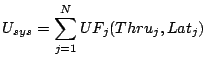 |
(2) |
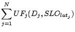
where  is the total number of workloads, is the total number of workloads,  is the utility function of workload
  , with throughput , with throughput  and
latency and
latency  . .
In addition, for any given workload demands  ,
the system maximum utility value ,
the system maximum utility value
 is defined as
the ``ideal'' maximum utility value if the requests for all workloads
are satisfied. Utility loss is defined as
the ``ideal'' maximum utility value if the requests for all workloads
are satisfied. Utility loss  is the difference
between the maximum utility value and the current system utility value. They
can be calculated as follows: is the difference
between the maximum utility value and the current system utility value. They
can be calculated as follows:
where the
 is the latency requirement of workload .
In addition, cumulative utility value for a given time window refers
to the sum of the utility value
across the time window. is the latency requirement of workload .
In addition, cumulative utility value for a given time window refers
to the sum of the utility value
across the time window.
These tools automate invocation of a single action.
A few examples are Chameleon [25],
Facade [17] for throttling;
QoSMig [10], Aqueduct [16] for migration;
Ergastulum [6], Hippodrome [5]
for
provisioning. Each of these tools typically includes the
logic for deciding the action invocation parameter values, and an executor to
enforce these parameters.
The single action tools take the system state, performance models and utility
functions as input from the Action Advisor and outputs the invocation parameters.
For example, in the case of migration, it decides the data to be migrated,
the target location, and the migration speed.
Every action has a cost
in terms of the resource or budget overhead and a benefit in
terms of the improvement in the performance of the workloads.
The action invocation parameters are used to determine the resulting
performance of each workload and the corresponding utility value.
The Action Advisor generates the corrective action schedule - the
steps involved are as follows (details of the algorithm are covered in
the next section):
- Generate and analyze the current state (
 ) as well as
lookahead states ( ) as well as
lookahead states (
 , ...) according
to the forecasted future. , ...) according
to the forecasted future.
- Feed the system states along with the workload utility functions and
performance models to the single action tools
and collect their invocation options
- Analyze the cost-benefit of the action invocation options -
this is accomplished using the Utility Evaluator module.
- Prune the solution space and generate a schedule of what
actions to invoke, when to invoke, and how to invoke.
3 Algorithm for Action Advisor in SMART
Action Advisor is the core of SMART: it determines
an action schedule consisting of one or more actions (what)
with action invocation time (when) and invocation parameters (how).
The goal of Action Advisor is to pick a combination of actions that will
improve the overall system utility or,
equivalently, reduce the system utility loss. In the rest of this section,
we will first intuitively motivate the algorithm and give the
details after that.
The Action Advisor operates in two different modes depending on whether
the corrective actions are being invoked proactively in response to
forecasted workload growth, or reactively in response to unexpected
variations in the workloads. The former is referred to as the
normal mode, while the later is the unexpected mode.
In the normal mode,
SMART uses an approach similar to the divide-and-conquer concept.
It breaks the optimization window into smaller unequal sub-windows and
uses a recursive greedy with look-back and look-forward approach to
select actions within each sub-window.The motivation of divide-and-conquer is to reduce the problem complexity
and to treat the near-term fine-grained prediction periods differently from
the long-term coarse-grained prediction periods.
The action selection for each sub-window is performed
in a sequential fashion, i.e., the resulting system state of one sub-window
acts as the starting state for the next consecutive window.
The divide-and-conquer approach reduces the problem complexity at
the cost of optimality: the sum of local optimal actions for each sub-window
may not lead to the global optimal.
The unexpected mode
selects actions defensively.
It tries to avoid
invoking expensive actions
since the workload variation could
go away soon after the action in invoked, making the overhead wasted. However this
needs to be balanced with the potential risk of the high workload
persisting and thus incurring continuous utility loss
which may add up over time.
We formulate this analysis as
a decision-making problem with unknown future
and apply the ``ski-rental'' online algorithm [15] to select actions.
Action Advisor uses a primitive mechanism to transition between
normal and unexpected modes. It continuously
compares the observed values against the predicted values (using any
chosen predictor model, for example, ARIMA). If the difference is
large then it moves into the defensive unexpected workload mode. While
in that mode, it continuously updates its predictor function based on
the newly observed values. When the predicted values and observed
values are close enough for a sufficiently
long period, it transitions to the normal mode.
In the rest of this section, we first present
action selections for normal mode and unexpected mode respectively.
After that, we discuss the risk modulation which deals with
the future uncertainty and action invocation overhead.
3.1 Normal Mode: Greedy Pruning with Look-back and Look-forward
The Action Advisor takes as input the current system state,
the workload prediction,
the utility functions,
the available budget  for new hardware and the length of the optimization window.
The action selection begins by breaking the specified optimization window into
smaller unequal sub-windows. For instance, a one year optimization window is
split into sub-windows of 1 day, 1 month, and 1 year;
The number and length of the sub-windows can be configured by the
administrator.
Within each sub-window for new hardware and the length of the optimization window.
The action selection begins by breaking the specified optimization window into
smaller unequal sub-windows. For instance, a one year optimization window is
split into sub-windows of 1 day, 1 month, and 1 year;
The number and length of the sub-windows can be configured by the
administrator.
Within each sub-window
![$ [T_{k},T_{k+1}]$](img38.png) , the goal is to find actions that maximize
the cumulative system utility
in the sub-window.
This process is formulated as a
tree-construction algorithm (Figure 3) as described
below. , the goal is to find actions that maximize
the cumulative system utility
in the sub-window.
This process is formulated as a
tree-construction algorithm (Figure 3) as described
below.
Figure 3:
Tree Based Action Schedule Generation
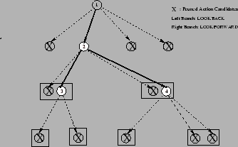 |
In the tree-based representation, the root corresponds to the entire
sub-window,
.
The branches originating from the root represent the candidate actions
returned by single action tools. For  possible action options
there will be branches. The resulting node possible action options
there will be branches. The resulting node  for each
action has the following information: for each
action has the following information:
- The selected action and its invocation parameters.
- The action invocation time and finish time
![$ [invoke_i, finish_i]$](img42.png) . .
- The decision window start and end time
![$ [start_i, end_i]$](img43.png) . For
nodes originating from the root, the value is . For
nodes originating from the root, the value is
![$ [T_k, T_{k+1}]$](img44.png) . .
- The initial
 and resulting state and resulting state
 . .
- The predicted cumulative utility loss
 , defined as the sum of
system utility loss from , defined as the sum of
system utility loss from  to to  if action is invoked. if action is invoked.
Greedy Pruning: Using the basic greedy approach, the Action Advisor selects a
first-level node in the tree that has the lowest utility loss and
prunes the other  branches (circles crossed out in Figure 3). In addition,
a threshold is introduced to ensure that the action gives
sufficient improvement. The selected action will only be scheduled
if the improvement exceeds the threshold.
The threshold is
configurable such that a higher value leads to more aggressive
pruning. This greedy pruning procedure is referred to as function GreedyPrune in
the pseudocode described later. branches (circles crossed out in Figure 3). In addition,
a threshold is introduced to ensure that the action gives
sufficient improvement. The selected action will only be scheduled
if the improvement exceeds the threshold.
The threshold is
configurable such that a higher value leads to more aggressive
pruning. This greedy pruning procedure is referred to as function GreedyPrune in
the pseudocode described later.
Lookback and Lookforward Optimization:
In real-world systems, it may be required to invoke more than one
action concurrently. For example, if data migration is selected, it
might be required to additionally throttle the lower priority
workloads until all data are migrated. The Action Advisor uses the
Look-back and Look-forward Optimization to improve the action plan.
The look-back and look-forward are with reference to the selected action's
finish time  . Look-back seeks action options in the time window . Look-back seeks action options in the time window
![$ [start_i, finish_i]$](img52.png) (before the selected action finishes).
Look-forward examines possible actions in the window
(before the selected action finishes).
Look-forward examines possible actions in the window
![$ [finish_i, end_i]$](img53.png) (after the selected action finishes).
Time is chosen as the splitting point because
(1) the system state is permanently changed after the action finishes,
making the cost-benefit of action options changed and (2)
any action scheduled before the selected action finishes need to satisfy the
no-conflict constraint (described later).
Essentially, the look-back and
look-forward optimization splits
the time window recursively and seeks actions to improve
the system utility further.
In the tree-construction, the action candidates for look-back
and look-forward are represented as left and right children (marked as
solid circles in Figure 3). The
pruning-lookback-lookforward procedure is recursively performed to
construct an action schedule until the GreedyPrune
finds no action option. The pseudocode for look-forward and look-back
optimization is given in function Lookback and Lookforward
respectively.
(after the selected action finishes).
Time is chosen as the splitting point because
(1) the system state is permanently changed after the action finishes,
making the cost-benefit of action options changed and (2)
any action scheduled before the selected action finishes need to satisfy the
no-conflict constraint (described later).
Essentially, the look-back and
look-forward optimization splits
the time window recursively and seeks actions to improve
the system utility further.
In the tree-construction, the action candidates for look-back
and look-forward are represented as left and right children (marked as
solid circles in Figure 3). The
pruning-lookback-lookforward procedure is recursively performed to
construct an action schedule until the GreedyPrune
finds no action option. The pseudocode for look-forward and look-back
optimization is given in function Lookback and Lookforward
respectively.
Function Lookback(i) {

  Foreach (Corrective_actions) {

    If (!(Conflict(Existing actions)) {

      Find action option in (start_i, finish_i);

      Add to Left_Children(i);

    }

  }

  GreedyPrune(Left_Children(i));

  If (Left_Children(i)!=NULL) {

     Lookback(Left_Children(i));

     Lookforward(Left_Children(i));

  }

}


Function Lookforward(i) {

  Foreach (Corrective_actions) {

    Find action option in (finish_i, end_i);

    Add to Right_Children(i);

  }

  GreedyPrune(Right_Children(i))

  If (Right_Children(i)!=NULL) {

     Lookback(Right_Children(i));

     Lookforward(Right_Children(i));

  }

}
When considering actions to be scheduled
before another action finishes (in lookback phase),
the actions should not conflict with existing selected
actions.
Two actions conflict if one of the following
is true:
- If they depend on the same resource.
- If action overlaps with an action
 already in the
schedule, and action violates the precondition for action .
For example, migration action 1 of moving data already in the
schedule, and action violates the precondition for action .
For example, migration action 1 of moving data  from from  to to
 will invalidate action 2 of moving data from
to will invalidate action 2 of moving data from
to  because the pre-condition of action 2 that data was on
is no longer true. because the pre-condition of action 2 that data was on
is no longer true.
In summary, the Action Advisor generates the schedule of corrective
actions using a recursive approach (the
pseudocode is given below). The final action schedule for each sub-window
is obtained by sorting the un-pruned nodes (solid circles in Figure 3)
in the tree according to their action invocation time ( ). ).
Function TreeSchedule() {

  Foreach (Corrective_actions) {

    Find action option in [T_k, T_{k+1}];

    Add to Children(root);

  }

  GreedyPrune(Children(root));

  If (Children(root) !=NULL) {

     Lookback(Children(root));

     Lookforward(Children(root));

  }

}
Finally, each sub-window is processed sequentially, i.e., the resulting
system state of sub-window
is the starting
state of sub-window
![$ [T_{k+1}, T_{k+2}]$](img60.png) , and the action schedules
are composed into the final action schedule according to the action invocation time. , and the action schedules
are composed into the final action schedule according to the action invocation time.
3.2 Unexpected Mode: Defensive Action Selection
Optimizing for the unexpected workload mode is challenging since it is
difficult to predict the duration for which workload variation will
persist. The Action Advisor uses a strategy similar to the one used in
on-line decision making scenarios such as the ``ski rental: to rent or to
buy'' [15]. There the choice of whether to buy (at cost say $150)
or rent a ski (at cost say $10 per trip) has to be made without the knowledge
of the future (how many times one might go skiing).
If one skis less than 15 times, then renting is
better, otherwise buying is better. In the absence of the knowledge of the
future, the commonly used strategy is ``to keep renting until the amount paid in
renting equals the cost of buying, and then buy.'' This strategy is always
within a factor of two of the optimal, regardless of how many times
one goes skiing, and is provably the best possible in the absence
of knowledge about the future.
The Action Advisor follows a similar online strategy. It selects the
least costly action until the cumulative utility loss for staying with
that action exceeds the cost of
invoking the next expensive action.
When SMART is in the unexpected
mode, the Action Advisor first finds
all action candidates under the assumption
that the system state
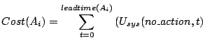
and workload demands will remain the same. For
each candidate  , the cost
is initialized as the extra utility loss and hardware cost (if
any) paid for the action invocation (shown in Equation 4): , the cost
is initialized as the extra utility loss and hardware cost (if
any) paid for the action invocation (shown in Equation 4):
 |
|
|
|
 |
|
|
(4) |
Where
 is the system utility value at time if
no corrective action is taken and
is the system utility value at time if
no corrective action is taken and
 is the system utility at time if is ongoing.
For example, for throttling,
is the system utility at time if is ongoing.
For example, for throttling,
 will be zero because the leadtime is
zero. For migration, the is
the total utility loss over will be zero because the leadtime is
zero. For migration, the is
the total utility loss over
 due to allocating resources to move data around.
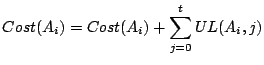
Action Advisor selects the action with minimum cost
and invokes it immediately. Over time,
the cost of each action candidate (including
both the selected one and unchosen ones)
is updated continuously to reflect the utility loss experienced
if had been invoked. Equation (5)
gives the value of after intervals:
 |
(5) |
This cost updating procedure continues until
following situations happen:
- Another action has a lower cost
than the previously invoked action. Action Advisor
invokes action immediately and continues
the cost updating procedure.
For example, if the system experiences
utility loss with throttling, but has no utility loss
after migration, the cost
for throttling action will continuously grow and
the cost of migration will stay same over time.
At some point, the cost of throttling will exceed the cost of migration
and the migration option will be invoked by then.
- System goes back to a good state for a period of time. The
Action Advisor will stop the action selection procedure
(exception has gone).
- The system collects enough new observations
and transitions back to normal mode.
In our previous discussion, action selection has been made
based on the cumulative utility loss .
The accuracy of depends on the accuracy of future workload
forecasting, performance prediction
and cost-benefit effect estimation of actions. Inaccurate estimation of
may result in decisions leading to reduced overall utility.
To account
for the impact of inaccurate input information, we perform risk modulation
on the for each action option. Here, risk captures both
the probability that the utility gain
of an action will be lost (in the future system-states) as a result of
volatility in the workload time-series functions (e.g., the demand for  was
expected to be was
expected to be  IOPS after 1 month, but it turns out to be IOPS after 1 month, but it turns out to be  , making
the utility improvement of buying new hardware wasted) and the impact of
making a wrong action decision (e.g., the impact of a wrong decision to migrate
data when the system is 90% utilized is higher than that of when the system is
20% loaded). , making
the utility improvement of buying new hardware wasted) and the impact of
making a wrong action decision (e.g., the impact of a wrong decision to migrate
data when the system is 90% utilized is higher than that of when the system is
20% loaded).
There are several techniques for measuring risk.
Actions for assigning storage
resources among workloads are analogous to portfolio management in
which funds are allocated to various company stocks. In
economics and finance,
the Value at Risk (VaR) [11] is a
technique used to estimate the probability of portfolio losses based
on the statistical analysis of historical price trends and
volatilities in trend prediction.
In the context of SMART,  represents
the probability with a 95% confidence, that the workload system will not
grow in the future, making the action invocation unnecessary. represents
the probability with a 95% confidence, that the workload system will not
grow in the future, making the action invocation unnecessary.
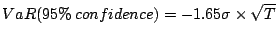 |
(6) |
where,
 is the standard deviation of the time-series
request-rate predictions and is the standard deviation of the time-series
request-rate predictions and  is the number of days in the future for which the risk
estimate holds. For different sub-windows, the prediction
standard deviation may be different: a near-term prediction is likely
to be more precise than a long-term one. is the number of days in the future for which the risk
estimate holds. For different sub-windows, the prediction
standard deviation may be different: a near-term prediction is likely
to be more precise than a long-term one.
The risk value  of action is calculated by: of action is calculated by:
 |
(7) |
where  reflects the risk factors of an individual action
(based on its operational semantics) and is defined as follows: reflects the risk factors of an individual action
(based on its operational semantics) and is defined as follows:
Where
 is the system utilization when the action is invoked. is the system utilization when the action is invoked.
For each action option returned by single action tools, the Action Advisor
calculates the risk factor and scales the
cumulative utility loss according to Equation 8 and
the action selection is performed based on the scaled
 (For example,
in GreedyPrune). (For example,
in GreedyPrune).
 |
(8) |
4 Experiments
SMART generates an action schedule to improve system utility. To
evaluate the quality of its decision, we implemented SMART in both
a real file system GPFS [21] and a simulator. System
implementation allows us to verify if SMART
can be applied practically while simulator
provides us a more controlled and
scalable environment, which allows
us to perform repeatable experiments to gain
insights on the overhead and sensitivity to
input information errors.
The experiments are divided into three parts:
First, sanity check experiments are performed
to examine
the impact of various configuration parameters on
SMART's decision.
Secondly, feasibility
experiments evaluate the behavior of two representative
cases in the sanity check using the GPFS prototype.
Third,
sensitivity test first examines the quality of the decisions
with accurate component models and future prediction over
a variety of scenarios using simulator. It then varies the error
rate of the component models and time series prediction
respectively and evaluates their impact on SMART's quality.
In addition, SMART is designed to assist the administrators to
make decisions. However, in order to examine the quality of SMART's decision (for example,
what will happen if the administrator follows SMART's advice),
selected actions are automatically executed
in the experiments.
In the rest of this section, we first
describe our GPFS prototype implementation
and then present the experimental results of three tests.
The SMART prototype is implemented on GPFS: a
commercial high-performance distributed file-system
[21]. GPFS manages the underlying
storage systems as pools that differ in their
characteristics of capacity, performance and availability.
The storage systems can be accessed by any clients
nodes running on separate physical machines
transparently.
The prototype implementation involved
sensors for monitoring the workloads states,
actuators for executing corrective actions and
an Action Advisor for decision making.
Sensors: They collect information about the run-time state of
workloads. The monitor daemon in each GPFS client node tracks the access
characteristics of the workload and writes it to a file, which can be analyzed
periodically in a centralized fashion.
Workloads are the unit of tracking and control - in the
prototype implementation, a workload is defined
manually as a collection of PIDs assigned by the OS. The monitoring
daemon does book-keeping at the GPFS read/write function call invoked after the
VFS translation.
Action actuators: Although the long
term goal of the prototype is to support all corrective actions,
as a proof of concept, we first implemented
action actuators for three most commonly used corrective actions:
throttling, migration and adding new pools.
- The IO throttling is enforced at
the GPFS client nodes using a token-bucket algorithm.
The decision-making for throttling each workload
is made in a centralized fashion, with the token-issue
rate and bucket
size written to a control file that is then periodically (20ms)
checked by the node throttling daemon.
- Similarly, the control file for the migration daemon consists
of entries of the form
 file name, source pool,
the destination pool file name, source pool,
the destination pool and the migration speed
is controlled by throttling the migration process.
The migration daemon thread runs in the context of one
of the client nodes and periodically checks
for updates in the control file and invokes
the GPFS built in function mmchattr
to migrate files. and the migration speed
is controlled by throttling the migration process.
The migration daemon thread runs in the context of one
of the client nodes and periodically checks
for updates in the control file and invokes
the GPFS built in function mmchattr
to migrate files.
- Because the addition of hardware normally
requires human intervention, we mimic the effect
of adding new hardware by pre-reserving storage
devices and forbidding the access to them
until SMART decides to add them into the system.
In addition,
the storage devices are configured
with different leadtime to mimic the overhead of placing orders
and installation.
In addition, the daemon threads for throttling and
migration run at the user-level and invoke kernel-level ioctls for the respective actions.
Action Advisor Integration:
The SMART action advisor is implemented using
techniques described in Section 3.
The time-series forecasting is done in an off-line fashion, where the monitored access characteristics for each
workload are periodically fed to the ARIMA module [24]
for refining the future forecast. Similarly, the performance
prediction is done by bootstrapping the system
for the initial models and refining the models
as more data are collected.
Once the Action Advisor is invoked,
it communicates with individual action
decision-making boxes
and generates an action schedule. The selected actions
are on hold by the action advisor until the
action invocation time (determined by SMART) is due.
At that time, the control files for corresponding
action actuators are updated according
to SMART's decision.
Without access to commercial decision tools, we implemented
our own throttling, migration and provisioning tools.
Throttling uses simulated annealing
algorithm [20] to allocate tokens for each
workload; the migration plan is generated by combining
optimization, planning and risk modulation. It
decides what and where
to migrate, when to start migration and migration speed. The provisioning decision
is done by estimating
the overall system utility for each provisioning option, which considers
the utility loss before the hardware
arrives, introduced by the load balancing operation (after
the new hardware comes into place) and the financial cost of buying
and maintaining the hardware.
As a sanity check, the action advisor in the GPFS prototype
is given the initial system settings as input, while the configuration parameters
are varied to examine their impact on SMART's action schedule.
The initial system setting for the tests is as follows:
Table 1:
Access characteristics of workloads
|
Workload |
Request size [KB] |
Rd/ wrt ratio |
Seq/ rnd ratio |
Foot-print [GB] |
ON/OFF phase [Hour] |
ON/OFF [Iops] |
 |
16 |
0.7 |
0.8 |
60 |
12/12 |
150/100 |
 |
16 |
1 |
1 |
600 |
8/16 |
250/0 |
 |
8 |
0.8 |
0.9 |
6 |
14/10 |
150/100 |
|
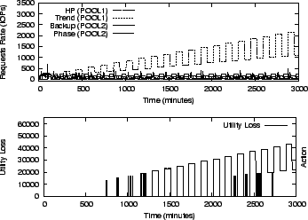
Workloads: There are four workload streams: one is
a 2 month trace replay of HP's Cello99
traces [18]. The other three workloads are
synthetic workload traces with the following characteristics: 1)
is a workload with a growth trend - the ON phase load
increases by 100 IOPS each day while the OFF phase load increases by
50 IOPS; 2) is a workload with periodic ON-OFF phases; 3)
simulates a backup load with its ON-phase as an inverse
of the phased workload. The access characteristics of these
workloads are summarized in Table
1. Figure 5 (a) shows the IO
rate of these workloads as a function of time. The default utility
function for violating and meeting the SLO latency goals are shown in
Figure 4
unless specified otherwise.
Figure 4:
(a) Utility functions for violating
SLO latency goals (b) Utility functions for meeting
SLO latency goals
 |
Components: There are three logical volumes:
POOL1 and POOL2 are both RAID 5 arrays with 16 drives each, while
POOL3 is a RAID 0 with 8 drives.
POOL3 is originally off-line, and is accessible only
when SMART selects hardware provisioning as a corrective action. The initial workload-to-component mapping is:
[HP: POOL1], [Trend: POOL1], [Phased: POOL2]
and [Backup: POOL2].
Miscellaneous settings: The optimization window is set to one
month; the default budget constraint is $20,000 and
the one day standard deviation of the load for risk
analysis is configured as 10% unless otherwise specified. The provisioning
tool is configured with 5 options, each with different buying cost, leadtime
and estimated performance models.
For these initial system settings, the system utility loss
at different time intervals without any corrective action
is shown in Figure 5 (b).
Figure 5:
(a) Workload Demands (b) utility loss if no corrective action is invoked
 |
An ideal yardstick to evaluate the quality of SMART's decisions is by
comparing it with existing automated algorithms or with decisions made
by an administrator. However, we are not aware of any existing work
that considers multiple actions; also, it is very difficult to
quantify decisions of a representative administrator. Because of this, we
take an alternative approach of comparing the impact of SMART's
decisions with the maximum theoretical system utility (upper bound, Equation 3)
and the system utility without any action (lower bound).
In the rest of this section, using the system settings described
above, we vary the configuration parameters that affect SMART's
scheduling decisions namely the utility function values (test
1); the length of optimization window (test 2), budget
constraints (test 3), risk factor (test 4). In test 5, we
explore how SMART handles unexpected case. For each of these tests, we
present the corrective action schedule generated by SMART, and the
corresponding predicted utility loss
as a function of time (depicted on the x-axis).
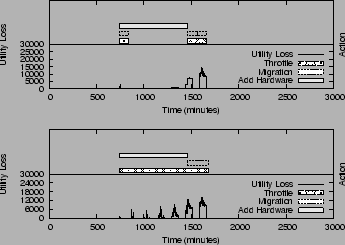
Test 1: Impact of Utility Function
Figure 6:
Action Invocation for different utility functions
assigned to  (a) Results for high utility value
 (default configuration) (b) Results for low
utility value assignment (default configuration) (b) Results for low
utility value assignment
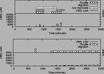 |
SMART selects actions that
maximize the overall system utility value, which is driven by the utility functions for
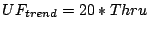
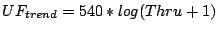
individual workloads using the storage system. In this test, we vary
's utility function of meeting the SLO latency
goal from the default  to to
 . As
shown in Figure 6(a), the default utility
assignment for causes a fast growing overall utility
loss - SMART selects to add new hardware. However, for
the low value utility assignment, the latency violation
caused by the increasing load results in a much slower
growth in the utility loss. As a result, the cost of adding
new hardware cannot be justified for the current optimization window and
hence SMART decides to settle for throttling
and migration. Note that as
the utility loss slowly approaches to the point where
the cost of adding new hardware can be justified,
SMART will suggest invoking hardware provisioning as needed. . As
shown in Figure 6(a), the default utility
assignment for causes a fast growing overall utility
loss - SMART selects to add new hardware. However, for
the low value utility assignment, the latency violation
caused by the increasing load results in a much slower
growth in the utility loss. As a result, the cost of adding
new hardware cannot be justified for the current optimization window and
hence SMART decides to settle for throttling
and migration. Note that as
the utility loss slowly approaches to the point where
the cost of adding new hardware can be justified,
SMART will suggest invoking hardware provisioning as needed.
Test 2: Impact of Optimization Window
Figure 7:
Action Invocation for different optimization windows
(a) Results for 2 days optimization window
(b) Results for 1 week optimization window
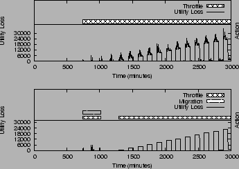 |
SMART is designed to select corrective actions that maximize the
overall utility for a given optimization window. In this test, we vary
the optimization window to 2 days, 1 week and 1 month (default value)
- compared to the schedule for 1 month in
Figure 6 (a), Figure 7 shows that
SMART correctively chooses different action schedules for the same
starting system settings. In brief, for a short optimization window
(Figure 7 (a) and (b)),
SMART correctly selects action options with a lower cost, while for a longer optimization window (Figure 6 (a)),
it suggests higher cost corrective options that are more beneficial in
the long run.
Test 3: Impact of Budget Constraints
Figure 8:
Action Invocation for different budget constraints
(a) no budget available (b) low budget ($5000)
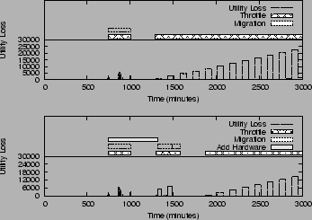 |
Test 3 demonstrates how SMART responds to various budget constraints.
As shown in Figure 8, SMART settles for throttling and
migration if
no budget is available for buying new hardware. With
$5000 budget, SMART opts for adding
a hardware. However,
compared to the hardware selected for the default $20,000 budget (shown
in Figure 6 (a)), the hardware selected is not
sufficient to solve the problem completely, and additionally requires a certain degree of traffic
regulation.
Test 4: Impact of Risk Modulation
Figure 9:
Action Invocation for different risk
factor. (a) Available migration option involves 20GB data movement (b) Available migration involves 1000GB data movement
 |
SMART uses risk modulation to balance between the risk of invoking an
inappropriate action and the corresponding benefit on the utility
value. For this experiment, the size of the dataset selected for
migration is varied, changing the risk value (Equation 7)
associated with the action options. SMART will select the high-risk
option only if its benefit is proportionally higher. As shown in
Figure 9, SMART changes the ranking of the
corrective options and selects a different action invocation schedule
for the two risk cases.
Test 5: Handling of Unexpected Case
Figure 10:
Action Invocation for unexpected case
(a) Workloads Demands (b) Result for a ``short'' spike (c)
results for a ``long'' spike
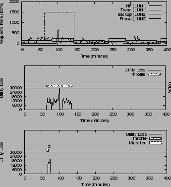 |
This test explores SMART's ability to handle the unexpected workload
demands. Figure 10 (a) shows the sending rate of
the workload demands.
From minute 60 to minute 145, sends
at 1500 IOPS instead of the normal 250 IOPS. The difference
between the predicted value 250 IOPS and the observed
value 1500 IOPS exceeds the threshold
and SMART switches to unexpected mode. For both
cases, SMART invokes throttling directly. But for case
1, the migration option involves a 1000 GB data movement and
is never invoked because
the spike duration is not long enough to reach
to a point where the migration invocation cost
is less than the utility loss of staying with throttling.
For case 2, a lower cost migration option is available (8GB data)
and after 5 minutes, the utility loss due to settling for throttling
already exceeds the invocation cost of migration.
The migration option is invoked immediately as a result.
In these tests, SMART is run within the actual GPFS deployment. The tests serve two purposes: (1) to verify if the action
schedule generated by SMART can actually help reduce system utility
loss; (2) to examine if the utility loss predicted by SMART
matches the observed utility loss. We run two
tests to demonstrate the normal mode and unexpected
mode operation.
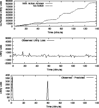
Test 1: Normal Model
Figure 11:
(a) cumulative utility loss comparison of
without action and with SMART's decision
(b) observed utility loss
(c) difference in Utility Loss (after filtering): Observed value-Predicted
 |
The setting for the experiment are the same as those used in the sanity
check tests with two exceptions: the footprint size, and the leadtime
of hardware addition. To reduce the experiment running time, the IO
features are changed to run 60 times faster (every minute in the
figure corresponds to one hour in the trace), and the footprint size
is shrunk by a factor of 60, and the leadtime of adding hardware is
set to 55 minutes (that maps to the original of 55 hours).
SMART evaluates the information and decides that the best
option is to add a new pool. Because
it takes 55 minutes to come into effect,
SMART looks back to seek for solutions
that can reduce the utility loss for time window [0, 55].
It chooses to migrate the  workloads from POOL1 to
POOL2 and throttle workloads
until the new pool arrives. After
POOL3 joins, the load balance
operation decides to migrate the workloads from POOL1 to
POOL2 and throttle workloads
until the new pool arrives. After
POOL3 joins, the load balance
operation decides to migrate the  workload
to POOL3 and back to POOL1. The final
workload to component mapping is: on POOL1, workload
to POOL3 and back to POOL1. The final
workload to component mapping is: on POOL1,  and
and  on POOL2 and on POOL3. on POOL2 and on POOL3.
As shown in Figure 11 (a),
compared to without any action,
SMART's action schedule eliminates about 80% of the original
utility loss and also grows at a much slower
rate. Before time 20, the no action utility
loss is slightly lower than with SMART
because the SMART schedule is paying extra
utility loss for invoking the migration operation.
It can be observed from Figure 11 (b) that
there is a negative utility loss. This is because the maximum utility is calculated based
on the planned workload demands, while the
observed utility value is calculated based on the
observed throughput. Due to the lack
of precise control in task scheduling, the workload
generator can not precisely generate I/O requests as
specified. For example: the workload generator for the HP traces
is supposed to send out requests at a rate of 57.46 IOPS at time 33
while the observed throughput is actually 58.59 IOPS. As a
result, the observed utility value is actually higher than
the maximum value and results in a negative utility loss.
For a similar reason, the observed utility loss fluctuates
very frequently around zero utility loss.
SMART schedules actions and predicts the
utility loss to be close to zero. However, the observed
utility loss (shown in Figure 11 (b)) has non-zero
values.
In order to understand the cause of this,
we filter out the amount of
observed utility loss due to imprecise workload generation (described above),
and plot the remaining utility loss
in Figure 11 (c).
As we can see, the predicted and observed values match
at most times except for two spikes at time 2 and time 58. Going
into the log of the run-time performance, we found
several high latency spikes ( +60ms compared to the normal 10ms)
on the migrated workload during migration. This is because
the migration process will lock 256 KB blocks for consistency purposes; hence
if the workload tries to access these blocks,
it will be delayed until the lock is released. The performance
models fail to capture this scenario and we observe
a mismatch between the predicted and observed utility values. However,
these are only transient behavior in the system and will not affect
the overall quality of SMART's decision.
Test 2: Unexpected Case
Figure 12:
Spike Case:
Cumulative Utility loss with migration invoked and without any action
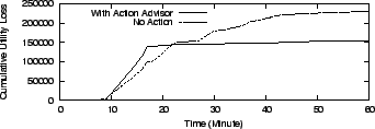 |
Similar to the sanity check test (Figure 10 (a)),
we intentionally create
a load surge from time 10 to time 50.
SMART invokes
throttling immediately and waits for about 3 minutes (time 13)
till the utility loss to invoke migration
is lower than the loss due to throttling.
The migration operation executed from time 13 to 17 and
the system experienced no utility loss once it was done.
Similar to the previous test, the temporarily
lesser utility loss without any action (shown in Figure 12)
is due to the extra utility loss
for data movement. We skip other figures due to a lack of
new observations for predicted and observed utility values.
We test the sensitivity of SMART on the errors
of performance prediction and future prediction in various
configurations.
This test is based on a simulator because it provides
a more controlled and scalable environment, allowing
us to test various system settings in a shorter time.
We developed a simulator
that takes the original system state, future
workload forecasting, performance models and
utility functions as input and simulates
the execution of SMART's decisions.
We vary the number of workloads in the system from 10 to 100.
For each workload setting, 50 scenarios are automatically generated as follows:
Workload features: The sending rate and footprint size
of each workload are generated using
Gaussian mixture distribution: with a high probability, the sending
rate (or footprint-size) is generated using a normal distribution with a lower mean value
and a low probability, it is generated using another
normal distribution with a larger mean value. The use of
Gaussian mixture distribution is to
mimic the real world behavior: a small
number of applications contributes a majority of the system load
and accesses the majority of data. Other workload characteristics are
randomly generated.
Initial data placement: the number of components
is proportional to the number of flows. For our tests,
it is randomly chosen to be 1/10 of the number of flows.
In addition, we intentionally
create an un-balanced system (60% of the workloads will go to one component
and the rest is distributed to other components randomly).
This
design is to introduce SLO violations and therefore,
utility loss such that corrective actions are needed.
Workload trending: In addition, to mimic workload
changes, 30% of workloads increases and 30% decreases.
In particular, the daily growing step size is generated using
a random distribution with mean of 1/10 of the original load and
the decreasing step size is randomly distributed with mean of 1/20
of the original load.
Utility functions: The utility function of meeting
the SLO requirement for each workload is assumed to be a linear
curve and the coefficients are randomly generated according to a uniform
distribution ranging from 5 to 50. The utility function of violating
the SLO requirement is assumed to be zero for all workloads. The
SLO goals are also randomly generated with considerations of the
workload demands and performance.
For a three month optimization window, the 500 scenarios experienced utility loss in various degrees
ranging from 0.02% to 83% of the maximum system utility (the
CDF is shown in Figure 13).
Test 1: With Accurate Performance Models and Future Prediction
Figure 13:
CDF of percentage of overall utility loss
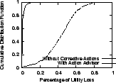 |
For this test, we assume both the performance prediction
and the future prediction are accurate. The Cumulative Distribution Functions of
the percentage of
utility loss (defined as
 )
for both with and without corrective actions
are shown in Figure 13. Comparing the two curves,
with actions selected by Action Advisor, SMART is very close to
the maximum utility. More than 80% scenarios
have a utility loss ratio less than 2% and more than 93%
have a ratio less than 4%. )
for both with and without corrective actions
are shown in Figure 13. Comparing the two curves,
with actions selected by Action Advisor, SMART is very close to
the maximum utility. More than 80% scenarios
have a utility loss ratio less than 2% and more than 93%
have a ratio less than 4%.
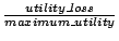
Test 2: With Performance Model Errors
Figure 14:
Impact of Model Errors
(a) Observed_Utility_Loss / Predicted_Utility_loss
(b) CDFs of Observed_Utility_Loss / Utility_Loss_Without_Action
 |
Our previous analysis is based on the assumption that perfectly
accurate component models are available for extrapolating latency for
a given workload. However, this is not always true in real-world
systems.
To understand how performance prediction errors affect the quality
of the decision, we perform the following experiments: (1) we generate a set of synthetic models and
make decisions based on them. The latency
calculated using these models is used as the ``predicted latency'' and
the corresponding utility loss is the ``predicted utility loss''. (2) For the
exact settings and action parameters, the ``real latency''
is simulated by adding errors on top of the ``predicted latency'' to
mimic the real system latency variations.
Because the residual normally grows with the real value,
we generate a random scaling factor rather than the absolute error.
For example, if the predicted latency is 10ms and the random error is 0.2,
the real latency is simulated as 10*(1+0.2) = 12ms. The ``real utility''
is estimated based on this.
Figure 14 (a) shows the ratio of
 ,
which reflects the degree of mismatch between the predicted and observed utility loss due to performance
prediction errors. As we can see, there is significant difference between
them - for a 20% model error, the average ,
which reflects the degree of mismatch between the predicted and observed utility loss due to performance
prediction errors. As we can see, there is significant difference between
them - for a 20% model error, the average
 is 6 times of the
predicted value. Next, we examine how does this difference affect the quality of the decision?
Figure 14(b)
plots the CDF of the remaining percentage of utility loss, defined as is 6 times of the
predicted value. Next, we examine how does this difference affect the quality of the decision?
Figure 14(b)
plots the CDF of the remaining percentage of utility loss, defined as
 .
It grows as the model error increases. But even with a 100% model error,
on average, the action selected by Action Advisor removes nearly 88% of the utility loss. .
It grows as the model error increases. But even with a 100% model error,
on average, the action selected by Action Advisor removes nearly 88% of the utility loss.
Test 3: With Time Series Prediction Errors
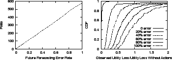
Figure 15:
Impact of Future Forecasting Errors
(a) Observed_Utility_Loss / Predicted_Utility_loss
(b) CDFs of Observed_Utility_Loss / Utility_Loss_Without_Action
 |
The future forecasting error is introduced in a similar fashion: the workload
demands forecasting is generated first. Based on that,
the ``real'' workload demands is generated by scaling with
a random factor following a normal distribution, with the future
forecasting error as the standard deviation. The predicted
utility loss is calculated based on the ``forecasted'' demands
and the observed utility loss is calculated based on the ``real''
workload demands. Note that, for this set of tests,
we restrict the Action Advisor only operating in the normal mode because otherwise,
Action Advisor will automatically switch to the unexpected mode.
Figure 15 (a) shows the ratio of the
to the
 . It is much bigger than
that of the model error: 560 vs 75 with 100% error. This is
because the future forecasting error has a larger scale.
For example, an error of under-estimating 10% of the future demands may
lead to 100 IOPS under-estimated, which may offset the performance prediction
even more than the one caused directly by model errors. Figure
15 (b) shows the CDF of remaining utility loss after invoking Action Advisor's action schedule.
It shows that as the future forecasting error grows, the probability
that the Action Advisor's decision is helpful reduces very quickly.
It can even result in
a utility loss higher than doing nothing. This confirms our design
choice: when the difference between the future prediction and observed values
are high, we should apply a defensive strategy rather than operating in
the normal mode. . It is much bigger than
that of the model error: 560 vs 75 with 100% error. This is
because the future forecasting error has a larger scale.
For example, an error of under-estimating 10% of the future demands may
lead to 100 IOPS under-estimated, which may offset the performance prediction
even more than the one caused directly by model errors. Figure
15 (b) shows the CDF of remaining utility loss after invoking Action Advisor's action schedule.
It shows that as the future forecasting error grows, the probability
that the Action Advisor's decision is helpful reduces very quickly.
It can even result in
a utility loss higher than doing nothing. This confirms our design
choice: when the difference between the future prediction and observed values
are high, we should apply a defensive strategy rather than operating in
the normal mode.
Comparing the results of model and future forecasting
errors, the quality of the decision
is more sensitive to future forecasting accuracy than to model
accuracy. In addition, we have used the ARIMA algorithm
to perform time-series analysis on HP's Cello99 real world trace
and the results show that more than 60% of the predictions falls
within 15% of the real value and more than 80% falls within
20%.
Storage virtualization can be host based [7], network
based [23] or storage controller based [28].
Storage virtualization can be at file level abstraction [13]
or block level abstraction [14]. These storage virtualization
solutions provide support for automatically extending volume size.
However, these virtualization solutions do not offer multi-action
based SLO enforcement mechanism and only recently single action based
(workload throttling)
SLO enforcement mechanisms are being combined with storage virtualization
solutions [9]. SLO enforcement can also be performed by
storage resource management software such as
control centerer from EMC [1] and total productivity
centerer from IBM [2].
These management software frameworks
provide sensor and actuator frameworks, and they
also have started to provide problem analysis and solution planning
functionality. However, the current versions of these
products do not have the ability to
combine multiple SLO enforcement mechanisms.
Research prototypes that provide single action based solutions
to handle SLO violations exist for a range of storage management
actions. Chameleon [25],
SLEDRunner [9],
and Facade [17]
prototypes provide workload throttling based SLO enforcement solutions.
QosMig [10] and Aqueduct [16] provide support
for data migration based SLO enforcement solutions.
Ergastulum [6], Appia [27] and Minerva [3]
are some capacity planning tools that can
be used to either design a new infra-structure or extend an existing
deployment in order to satisfy SLOs.
Hippodrome [5] is a feedback based storage management
framework from HP that monitors system behavior and
comes up with a strategy to migrate the system from the current state to the
desired state. Hippodrome focuses on migrating data and
re-configuring the system to transform it from
its current state to the new desired state.
6 Conclusion and Future Work
SMART generates a combination of corrective actions. Its action
selection algorithm considers a variety of information including
forecasted system state, action cost-benefit effect estimation
and business constraints, and generates an action schedule that can
reduce the system utility loss. It also can generate action plans
for different optimization windows and react to both expected load surges
and unexpected ones.
SMART's prototype has been implemented in a file system.
Our experiments show that the system utility value
is improved as predicted. Experimental results show that
SMART's action decision can result in less than 4% of utility loss.
Finally,
it is important to note that this framework can also be deployed as part
of storage resource management software or storage virtualization software.
Currently, we are designing
a robust feedback mechanism to handle various uncertainties in production
systems. We are also developing pruning techniques to reduce
the decision making overhead, making SMART applicable in large data center
and scientific deployments.
We want to thank John Palmer for his insights and comments on earlier versions of this paper.
We also want to thank the anonymous reviewers for their valuable comments. Finally,
we thank the HP Labs Storage Systems Department for making their traces available to the general public.
- 1
-
EMC ControlCenter family of storage resource management (SRM).
https://www.emc.com/
products/storage_management/controlcenter.jsp.
- 2
-
IBM TotalStorage.
https://www-1.ibm.com/servers/storage.
- 3
-
ALVAREZ, G. A., BOROWSKY, E., GO, S., ROMER, T. H., BECKER-SZENDY, R.,
GOLDING, R., MERCHANT, A., SPASOJEVIC, M., VEITCH, A., AND WILKES, J.
Minerva: An automated resource provisioning tool for large-scale
storage systems.
ACM Transactions on Computer Systems 19, 4 (2001), 483-518.
- 4
-
ANDERSON, E.
Simple table-based modeling of storage devices.
Tech. Rep. HPL-SSP-2001-4, HP Laboratories, July 2001.
- 5
-
ANDERSON, E., HOBBS, M., KEETON, K., SPENCE, S., UYSAL, M., AND VEITCH,
A.
Hippodrome: Running circles around storage administration.
Proceedings of Conference on File and Storage Technologies
(FAST) (Jan. 2002), 175-188.
- 6
-
ANDERSON, E., KALLAHALLA, M., SPENCE, S., SWAMINATHAN, R., AND WANG, Q.
Ergastulum: an approach to solving the workload and device
configuration problem.
Tech. Rep. HPL-SSP-2001-5, HP Laboratories, July 2001.
- 7
-
ANONYMOUS.
Features of veritas volume manager for unix and veritas file system.
https://www.veritas.com/us/products/volumemanager/whitepaper-02.html
(2005).
- 8
-
AZOFF, M. E.
Neural network time series forecasting of financial markets.
- 9
-
CHAMBLISS, D., ALVAREZ, G. A., PANDEY, P., JADAV, D., XU, J., MENON, R.,
AND LEE, T.
Performance virtualization for large-scale storage systems.
Proceedings of the 22nd Symposium on Reliable Distributed
Systems (Oct. 2003), 109-118.
- 10
-
DASGUPTA, K., GHOSAL, S., JAIN, R., SHARMA, U., AND VERMA, A.
Qosmig: Adaptive rate-controlled migration of bulk data in storage
systems.
ICDE (2005).
- 11
-
DIEBOLD, F.X., SCHUERMANN, T., AND STROUGHAIR, J.
Pitfalls and oppotunities in the use of extreme value theory in risk
management.
- 12
-
GANGER, G. R., WORTHINGTON, Y. N., AND PATT, B. L. A.
The DiskSim simulation environment version 1.0 reference manual.
Tech. Rep. CSE-TR-358-98, 27 1998.
- 13
-
GHEMAWAT, S., GOBIOFF, H., AND LEUNG, S.-T.
Google file system.
Proceedings of SOSP (2003).
- 14
-
GLIDER, J., FUENTE, F., AND SCALES, W.
The software architecture of a san storage control system.
IBM System Journal 42, 2 (2003), 232-249.
- 15
-
KARP, R.
On-line algorithms versus off-line algorithms: how much is it worth
to know the future?
In Proceedings of IFIP 12th World Computer Congress (1992),
vol. 1, pp. 416-429.
- 16
-
LU, C., ALVAREZ, G. A., AND WILKES, J.
Aqueduct: online data migration with performance guarantees.
Proceedings of Conference on File and Storage Technologies
(FAST) (Jan. 2002), 175-188.
- 17
-
LUMB, C., MERCHANT, A., AND ALVAREZ, G.
Facade: Virtual storage devices with performance guarantees.
Proceedings of 2nd Conference on File and Storage Technologies
(FAST) (Apr. 2003), 131-144.
- 18
-
RUEMMLER, C., AND WILKES, J.
A trace-driven analysis of disk working set sizes.
Tech. Rep. HPL-OSR-93-23, Palo Alto, CA, USA, May 1993.
- 19
-
RUEMMLER, C., AND WILKES, J.
An introduction to disk drive modeling.
Computer 27, 3 (1994), 17-28.
- 20
-
RUSSELL, S., AND NORVIG, P.
Artificial Intelligence A Modern Approach.
Prentice Hall, 2003.
- 21
-
SCHMUCK, F., AND HASKIN, R.
Gpfs: A shared disk file system for large computing clusters, 2002.
- 22
-
SHRIVER, E., MERCHANT, A., AND WILKES, J.
An analytic behavior model for disk drives with readahead caches and
request reordering.
In Proceedings of the 1998 ACM SIGMETRICS joint international
conference on Measurement and modeling of computer systems (New York, NY,
USA, 1998), ACM Press, pp. 182-191.
- 23
-
TATE, J., BOGARD, N., AND JAHN, T.
Implementing the ibm totalstorage san volume controller software on
the cisco mds 9000.
IBM Redbook SG24-7059-00 (2004).
- 24
-
TRAN, N., AND REED, D. A.
ARIMA time series modeling and forecasting for adaptive i/o
prefetching.
Proceedings of the 15th international conference on
Supercomputing (2001), 473-485.
- 25
-
UTTAMCHANDANI, S., YIN, L., ALVAREZ, G., PALMER, J., AND AGHA, G.
Chameleon: a self-evolving, fully-adaptive resource arbitrator for
storage systems.
Proceeding of Usenix Annual Technical Conference (Usenix)
(June 2005).
- 26
-
WANG, M., AU, K., AILAMAKI, A., BROCKWELL, A., FALOUTSOS, C., AND GANGER,
G. R.
Storage device performance prediction with CART models.
SIGMETRICS Perform. Eval. Rev. 32, 1 (2004), 412-413.
- 27
-
WARD, J., O'SULLIVAN, M., SHAHOURNIAN, T., WILKES, J., WU, R., AND BEYER,
D.
Appia and the hp san designer: automatic storage area network fabric
design.
In HP Technical Conference (Apr. 2003).
- 28
-
WARRICK, C., ALLUIS, O., AND ETAL.
The ibm totalstorage ds8000 series: Concepts and architecture.
IBM Redbook SG24-6452-00 (2005).
- 29
-
WILKES, J.
The pantheon storage-system simulator.
Tech. Rep. HPL-SSP-95-14, HP Laboratories, dec 1995.
SMART: An Integrated Multi-Action Advisor for Storage Systems
This document was generated using the
LaTeX2HTML translator Version 2002-2-1 (1.70)
Copyright © 1993, 1994, 1995, 1996,
Nikos Drakos,
Computer Based Learning Unit, University of Leeds.
Copyright © 1997, 1998, 1999,
Ross Moore,
Mathematics Department, Macquarie University, Sydney.
The command line arguments were:
latex2html -split 0 -show_section_numbers -local_icons paper.tex
The translation was initiated by Li Yin on 2006-04-17
Li Yin
2006-04-17
|