Check out the new USENIX Web site. next up previous
Next: Average vs. Worst-case Execution Up: Performance Evaluation Previous: Performance Evaluation


Experiment Setup

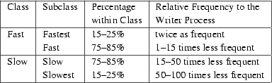
The algorithms we evaluate in this section are implemented and executed under EMERALDS OS [35] running on a Pentium-III 500Mhz processor. The experiments use a synthetic reader task set, which is divided into two sets -- fast readers and slow readers, where `fast' and `slow' are defined relative to the writer's period. In a real system, there are usually tasks that are executed very frequently, and tasks that run very infrequently. To model this behavior, we further divide the fast and slow reader sets into finer-grained categories, as shown in Figure 11. By making approximately 20% of fast and slow readers either very fast or very slow, the resulting task set represents realistic range of task periods that may occur in a real-time embedded system. A random reader task set is generated for each experiment according to the desired division of readers into the four categories.

Figure: Reader task set distribution.
\begin{figure}\begin{tabular}{\vert l\vert l\vert l\vert l\vert} \cline{1-4}
{\s...
...25\%} & {\small 50-100 times less
frequent} \ \hline
\end{tabular}\end{figure}

\begin{figure*}\epsfig{figure=./fig/mlegend.eps,width=7in,height=.3in,clip=}\end{figure*}

Figure: The top and bottom rows show the average-case and worst-case execution times, respectively, of the SMP version of the algorithms, to perform an IPC read / write operation with 8-byte message size.
\begin{figure*}\begin{tabular}{c c c c}
{\epsfig{figure=./fig/m8t20.eps,width=1....
... 12 fast readers & \small (h) 4 slow, 16 fast readers
\end{tabular}\end{figure*}

\begin{figure*}\epsfig{figure=./fig/ulegend.eps,width=7in,height=.3in,clip=}\end{figure*}

Figure: The top and bottom rows show the average-case and worst-case execution times, respectively, of the uniprocessor version of the algorithms, to perform an IPC read / write operation with 8-byte message size.
\begin{figure*}\begin{tabular}{c c c c}
{\epsfig{figure=./fig/u8t20.eps,width=1....
... 12 fast readers & \small (h) 4 slow, 16 fast readers
\end{tabular}\end{figure*}

\begin{figure*}\epsfig{figure=./fig/ulegend.eps,width=7in,height=.3in,clip=}\end{figure*}

Figure: These graphs show the space requirements for different algorithms with 8-byte messages (note that the space requirement is architecture-independent).
\begin{figure*}\begin{tabular}{c c c c}
\\
{\epsfig{figure=./fig/u8s20.eps,widt...
... 12 fast readers & \small (d) 4 slow, 16 fast readers
\end{tabular}\end{figure*}


next up previous
Next: Average vs. Worst-case Execution Up: Performance Evaluation Previous: Performance Evaluation
hai huang 2002-03-30