Choosing $r$ and $t$ for Each Test Load

The runlength $r$ and the number of trials $t$ together determine the benchmarking cost incurred at a given test load $\lambda$. The controller should choose $r$ and $t$ to obtain the confidence and accuracy desired for each test load at least cost. The goal is to converge quickly to an accurate reading at the peak rate: $\lambda = \lambda^*$ and load factor $\rho = 1$. High confidence and accuracy are needed for the final test load at $\lambda = \lambda^*$, but accuracy is less crucial during the search for the peak rate. Thus the controller has an opportunity to reduce benchmarking cost by adapting the target confidence and accuracy for each test load $\lambda$ as the search progresses, and choosing $r$ and $t$ for each $\lambda$ appropriately.

At any given load level the controller can trade off confidence and accuracy for lower cost by decreasing either $r$ or $t$ or both. Also, at a given cost any given set of trials and runlengths can give a high-confidence result with wide confidence intervals (low accuracy), or a narrower confidence interval (higher accuracy) with lower confidence.

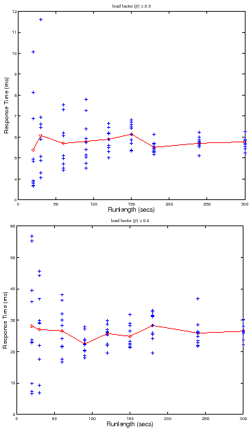
However, there is a complication: performance variability tends to increase as the load factor $\rho$ approaches saturation. Figure 4 and Figure 5 illustrate this effect. Figure 4 is a scatter plot of mean server response time ($\bar{R}$) at different test loads $\lambda$ for five trials at each load. Note that the variability across multiple trials increases as $\lambda \rightarrow \lambda^*$ and $\rho \rightarrow 1$. Figure 5 shows a scatter plot of $\bar{R}$ measures for multiple runlengths at two load factors, $\rho = 0.3$ and $\rho = 0.9$. Longer runlengths show less variability at any load factor, but for a given runlength, the variability is higher at the higher load factor. Thus the cost for any level of confidence and/or accuracy also depends on load level: since variability increases at higher load factors, it requires longer runlengths $r$ and/or a larger number of trials $t$ to reach a target level of confidence and accuracy.

For example, consider the set of trials plotted in Figure 5. At load factor $0.3$ and runlength of $90$ seconds, the data gives us $70$% confidence that $5.6 < \bar{R} < 6$, or $95$% confidence that $5 < \bar{R} < 6.5$. From the data we can determine the runlength needed to achieve target confidence and accuracy at this load level and number of trials $t$: a runlength of $90$ seconds achieves an accuracy of $87$% with $95$% confidence, but it takes a runlength of $300$ seconds to achieve $95$% accuracy with $95$% confidence. Accuracy and confidence decrease with higher load factors. For example, at load factor $0.9$ and runlength $90$, the data gives us $70$% confidence that $21 < \bar{R} < 24$ ($93.3$% accuracy), or $95$% confidence that $20 < \bar{R} < 27$ ($85.1$% accuracy). As a result, we must increase the runlength and/or the number of trials to maintain target levels of confidence and accuracy as load factors increase. For example, we need a runlength of $120$ seconds or more to achieve accuracy $\geq 87$% at $95$% confidence for this number of trials at load factor $0.9$.

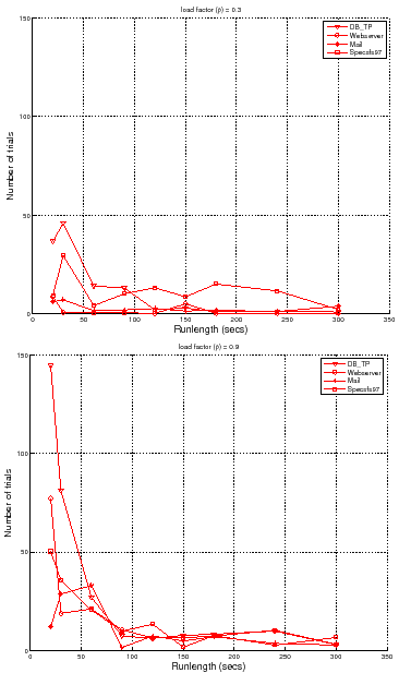
Figure 6 quantifies the tradeoff between the runlength and the number of trials required to attain a target accuracy and confidence for different workloads and load factors. It shows the number of trials required to meet an accuracy of $90$% at $95$% confidence level for different runlengths. The figure shows that to attain a target accuracy and confidence, one needs to conduct more independent trials at shorter runlengths. It also shows a sweet spot for the runlengths that reduces the number of trials needed. A controller can use such curves as a guide to pick a suitable runlength $r$ and number of trials $t$ with low cost.

Figure: Mean server response time $\bar{R}$ at different workload runlengths for the DB_TP fstress workload using $1$ disk and $4$ NFS daemon (nfsd) threads for the server. The variability in mean server response time for multiple trials decreases with increase in runlength. The results are representative of other server configurations and workloads.

Figure 6: Number of trials to attain $90$% accuracy for mean server response time at $95$% confidence level at low and high load factors for different runlengths. The results are for server configuration with $1$ disk and $4$ nfsds, and representative of other server configurations.