The replica selection algorithm used in Web++ is an extension of the Refresh algorithm studied in [35]. The Web++implementation of the Refresh algorithm extends the original algorithm in a number of ways:
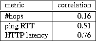
We chose to minimize the response time perceived by the end-user because this is the metric perceived by the end-user. Consequently, the HTTP request response time would be an ideal metric for selection of a ``nearby'' server. However, the response time depends also on resource size, which is unknown at the time of a request submission. Therefore, the HTTP request response time needs to be estimated using some other metric. We chose the HTTP request latency, i.e., the time to receive the first byte of the request, because we found that it is well correlated with the HTTP request response time as shown in Figure 3. The results in Figure 3 are based on client-side proxy traces collected in the computer lab of Northwestern University and further described in [35].
We chose a combination of active and passive measurement of HTTP request latency. Namely, most of the time clients passively reuse the statistics they collected from previously sent requests. However, periodically, clients actively poll some of the servers that have not been used for a long time. Each Web++ client applet collects statistics about the latencies observed for each server and keeps them in a latency table, which is persistently stored on a local disk. To increase the sampling frequency perceived by any individual client, the latency table is shared by multiple clients. In particular, the latency table is stored in a shared file system and is accessible to all clients using the file system3. We have implemented a rudimentary concurrency control mechanism to provide access to the shared latency table. Namely, the table is locked when clients synchronize their memory based copy with the disk based shared latency table. The concurrency control guarantees internal consistency of the table, but does not prevent lost updates. We believe that such a permissive concurrency control is adequate given that the latency table content is interpreted only as a statistical hint. The importance of sharing statistical data for clients using passive measurements has been pointed out in [38].
The estimate of the latency average, which is kept in the latency table, is used to predict the response time of a new request sent to a server. However, should two servers have similar average latencies, the latency variance should be used to break the tie, because it estimates the quality of service provided by a given server. There are several ways to combine the average and variance into a single metric. We chose a percentile because unlike e.g. statistical hypothesis testing it always provides an ordering among the alternatives.
An S-percentile is recursively estimated as
The average avgnew is estimated using a recursive formula
The number of samples that affect the estimates in (2) and
(3) continuously grows. Consequently, the importance of
variance in (1) would decrease in time. However, the samples
in (2) and (3) are exponentially weighted, so only a
small fixed number of most recent samples affects the current
estimates. Namely, the recursive formula for average (2) can be
expanded as
| (5) |
Our extended Refresh algorithm selects the server with the minimum S-percentile of latency. Unfortunately, a straightforward implementation of a replica selection algorithm that selects resource replicas solely based on latencies of requests previously sent to the server holding the selected replica leads to a form of starvation. In particular, the replica selection is based on progressively more and more stale information about the replicas on servers that are not selected for serving requests. In fact, it has been shown that in many cases a random decision is better than a decision based on too old information [33]. There are several possibilities for implementing a mechanism for ``refreshing'' the latency information for the servers that have not been contacted in a long time. One possibility is to make the selection probabilistic, where the probability that a replica is selected is inversely proportional to HTTP request latency estimate for its server. An advantage of such a mechanism is that it does not generate any extra requests. However, the probabilistic selection leads also to performance degradation as shown in [35] because some requests are satisfied from servers that are known to be sub-optimal. We, therefore, chose a different approach where the client applet refreshes its latency information for each server with the most recent sample that is older than time-to-live (TTL) minutes. The refreshment is done by sending an asynchronous HEAD request to the server. Therefore, the latency estimate refreshment does not impact the response time perceived by the user. On the other hand, the asynchronous samples lead to an extra network traffic. However, the volume of such traffic can be explicitly controlled by setting the parameter TTL.
Upon sending a request to a server, the client applet sets a timeout. If the timeout expires, the applet considers the original server as failed and selects the resource on the best server among the remaining servers that replicate the resource. The timeout should reflect the response time of the server. For example, a server located overseas should have a higher timeout than a server located within the same WAN. We chose to set the timeout to a T-percentile of request latency in order to reuse the statistical information collected for other purposes. T is a system parameter and typically should be set relatively high (e.g. 99) in order to base the timeout on a pessimistic estimate.
After the timeout for a request sent to a server expires, the applet marks the server entry in the latency table as ``failed''. For every ``failed'' server, the applet keeps polling the server by asynchronously sending a HEAD request for a randomly chosen resource every F seconds until a response is received. Initially, F is set to a default value that can be for example the mean time-to-repair (MTTR) of Internet servers measured in [29]. Subsequently, the value of F is doubled each time an asynchronous probe is sent to the server. After receiving a response, the value of F is reset to its default value. The default value of F is a system parameter. The pseudo-code of the replica selection algorithm can be found in Figure 4.
Input: d - requested resource |