Impact of multiple ISPs on circuitousness

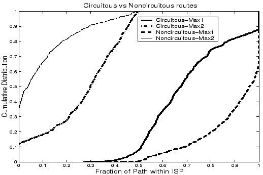
Figure 11: CDF of the fraction of the end-to-end path that lies within the top 2 ISPs in the case of circuitous paths and non-circuitous paths.

In Section 5.1 we hypothesized that the presence of multiple ISPs in an end-to-end path contributes to the circuitousness of the path. We now examine this issue more carefully. We classify end-to-end paths into two categories - non-circuitous (distance ratio $<$ 1.5) and circuitous (distance ratio $>$ 2).⁷ For each path in either category, we identify the top two ISPs that account for most of the end-to-end linearized distance. We then compute the fraction of the end-to-end linearized distance that is accounted for by the top two ISPs, and denote these fractions by $\max_1$ and $\max_2$. For example, if an end-to-end path with a linearized distance of 1000 km traverses 400 km in AT&T's network and 300 km in UUNET's network (and smaller distances in other networks), then $\max_1 = 0.4$ and $\max_2=0.3$. Note that it is possible for $\max_1$ to be 1.0 (and so $\max_2$ to be 0.0) if the entire end-to-end path traverses just one ISP network. We note that local-area networks confined to a city (e.g., a university network) contribute nil to the linearized distance and therefore are ignored. Figure 11 shows the CDF of $\max_1$ and $\max_2$ for the circuitous and non-circuitous paths. The difference in the characteristics of these two categories of paths is striking. The $\max_1$ and $\max_2$ curves are much closer together in the case of circuitous paths than in the case of non-circuitous paths. In other words, in the case of circuitous paths, the end-to-end path traverses substantial distances in each of the top two ISPs (and perhaps other ISPs too). In contrast, non-circuitous paths tend to be dominated by a single ISP. For instance, the median values of $\max_1$ and $\max_2$ in the case of circuitous paths is approximately 0.65 and 0.3, respectively. In other words, the top two ISPs account for 65% and 30%, respectively, of the end-to-end path in the median case. However, the fractions for the non-circuitous paths are approximately 95% and 4%, respectively - much more skewed in favor of the top ISP.

Figure 12: CDF of the distance ratio as a function of the number of major ISPs traversed along an end-to-end path. There were few paths that traversed more than 3 major ISPs.

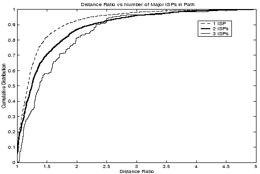We also consider the impact of the number of major ISPs traversed along an end-to-end path on the distance ratio. Figure 12 shows a clear trend: the distance ratio tends to increase as the path traverses a greater number of ISPs. For instance, the median distance ratios are 1.18, 1.25, and 1.38, respectively with 1, 2, and 3 major ISPs. The 90th percentile of the distance ratio is 1.81, 2.26, and 2.35, respectively. A path that traverses a larger number of major ISPs may span a greater distance. However, as noted in Section 5.1.1, this would not explain the larger distance ratio. In fact, a greater geographic distance would tend to make the distance ratio smaller, not larger These findings reinforce our hypothesis that there is a correlation between the circuitousness of a path (as quantified by the distance ratio) and the presence or absence of multiple ISPs that account for substantial portions of the path.