


Next: Access Frequency
Up: Server Access Pattern
Previous: Server Access Pattern
The first part of our study explored the temporal locality of server
buffer cache accesses. Past studies have shown that client buffer
cache accesses exhibit a high degree of spatial and temporal locality.
An accessed block exhibits temporal locality if it is likely to
be accessed again in the near future. An accessed block exhibits spatial
locality, if blocks near it are likely to be
accessed in the near future [11,38]. The LRU
replacement algorithm, typically used in client buffer caches,
takes advantage of temporal locality. Thus, blocks with a
high degree of temporal locality are likely to remain in a client
buffer cache, but accesses to a server buffer cache are misses from a
client buffer cache. Do server buffer cache acccesses exhibit temporal
locality similar to those of a client buffer cache?
We used temporal distance histograms to observe the temporal
locality of the server buffer cache traces. A reference sequence
(or reference string) is a numbered sequence of temporally
ordered accesses to a server buffer cache. The temporal distance
is the distance between two accesses to the same block in the
reference sequence. It is similar to the inter-reference gap
in [30]. For example, in the reference sequence  ,
the temporal distance from
,
the temporal distance from  to
to  is 5 and the temporal
distance from
is 5 and the temporal
distance from  to
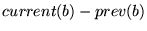
to  is 3. Formally speaking, if we denote
the sequence number of the current access and previous access to a
block
is 3. Formally speaking, if we denote
the sequence number of the current access and previous access to a
block  as
as  and
and  respectively, then the
temporal distance of the current access to block is
respectively, then the
temporal distance of the current access to block is
 . A temporal distance histogram shows how many
correlated accesses (accesses to the same block) for various temporal
distances reside in a given reference sequence.
. A temporal distance histogram shows how many
correlated accesses (accesses to the same block) for various temporal
distances reside in a given reference sequence.
Figure 2:
Comparison of temporal locality of client and server buffer cache
accesses using temporal distance histograms. (Note: figures are in
different scales)
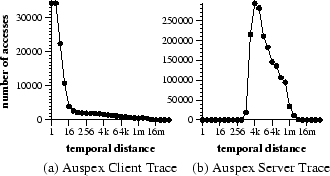 |
Figure 3:
Temporal distance histograms of server buffer cache accesses
for different traces. (Note: figures are in different scales)
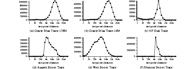 |
Figure 2 compares the client and server buffer cache's
temporal locality using temporal distance histograms with the Auspex
traces. The client buffer cache trace is collected at an Auspex
client, while the server buffer cache trace is captured at the Auspex
File Server. Each Auspex client uses an 8 megabyte buffer cache. The
data in the figure shows the histograms by grouping temporal distances
by powers of two. The block size is 8 Kbytes. Results are similar with
other block sizes. Distances that are not a power of two are rounded
up to the nearest power of two. Significantly, for the client buffer
cache 74% of the correlated references have a temporal distance less
than or equal to 16. This indicates a high degree of temporal
locality. Even more significantly, however, 99% of the correlated
accesses to the server buffer cache have a temporal distance of 512 or
greater, exhibiting much weaker temporal locality.
Figure 3 shows the temporal distance histograms of four
server buffer cache traces. These traces exhibit two common patterns.
First, all histogram curves are hill-shaped. Second, peak temporal
distance values, while different, are all relatively large and occur
at distances greater than their client cache sizes (see
Table 1). This access behavior at server buffer
caches is expectable. If a client buffer cache of size  uses
an locality-based replacement policy, after a reference to a block, it
takes at least references to evict this block from the client
buffer cache. Thus, subsequent accesses to the server buffer cache
should be separated by at least non-correlated references in the
server buffer cache reference sequence.
A good replacement algorithm for server buffer caches should retain
blocks that reside in the ``hill'' portion of the histogram for a
longer period of time. In this paper, ``time'' means logical time, measured by the
number of references. For example, initially, time is 0, after
accesses
uses
an locality-based replacement policy, after a reference to a block, it
takes at least references to evict this block from the client
buffer cache. Thus, subsequent accesses to the server buffer cache
should be separated by at least non-correlated references in the
server buffer cache reference sequence.
A good replacement algorithm for server buffer caches should retain
blocks that reside in the ``hill'' portion of the histogram for a
longer period of time. In this paper, ``time'' means logical time, measured by the
number of references. For example, initially, time is 0, after
accesses  , time is 3. We call the beginning and end of this ``hill''
region minimal distance (or
, time is 3. We call the beginning and end of this ``hill''
region minimal distance (or  ) and maximal
distance (or
) and maximal
distance (or  ) respectively. We picked and
for each trace by examining the histogram figure for
simplicity. Since the temporal distance values in the ``hill'' are
relatively large, a good replacement algorithm should keep most blocks
in this region for at least the time. We call this property
minimal lifetime property. It is clear that when the number of
blocks in a server buffer cache is less than the of a given
workload, the LRU policy tends to perform poorly, because most blocks
do not stay in the server buffer cache long enough for subsequent
correlated accesses.
) respectively. We picked and
for each trace by examining the histogram figure for
simplicity. Since the temporal distance values in the ``hill'' are
relatively large, a good replacement algorithm should keep most blocks
in this region for at least the time. We call this property
minimal lifetime property. It is clear that when the number of
blocks in a server buffer cache is less than the of a given
workload, the LRU policy tends to perform poorly, because most blocks
do not stay in the server buffer cache long enough for subsequent
correlated accesses.
Next: Access Frequency
Up: Server Access Pattern
Previous: Server Access Pattern
Yuanyuan Zhou
2001-04-29