Title

Niels Provos
Center for Information Technology Integration
University of Michigan
provos@citi.umich.edu

Abstract:

The main purpose of steganography is to hide the occurrence of communication. While most methods in use today are invisible to an observer's senses, mathematical analysis may reveal statistical anomalies in the stego medium. These discrepancies expose the fact that hidden communication is happening.

This paper presents improved methods for information hiding. One method uses probabilistic embedding to minimize modifications to the cover medium. Another method employs error-correcting codes, which allow the embedding process to choose which bits to modify in a way that decreases the likelihood of being detected. In addition, we can hide multiple data sets in the same cover medium to provide plausible deniability.

To prevent detection by statistical tests, we preserve the statistical properties of the cover medium. After applying a correcting transform to an image, statistical steganalysis is no longer able to detect the presence of steganography. We present an a priori estimate to determine the amount of data that can be hidden in the image while still being able to maintain frequency count based statistics. This way, we can quickly choose an image in which a message of a given size can be hidden safely. To evaluate the effectiveness of our approach, we present statistical tests for the JPEG image format and explain how our new method defeats them.

Introduction

Steganography is the art and science of hiding the fact that communication is taking place. While classical steganographic systems depend on keeping the encoding system secret, modern steganography tries to be undetectable unless secret information is known, namely, a secret key. Because of their invasive nature, steganographic systems leave detectable traces within a medium's characteristics. This allows an eavesdropper to detect media that have been modified, revealing that secret communication is taking place. Although the secret content is not exposed, its hidden nature is revealed, which defeats the main purpose of steganography.

In general, the information hiding process starts by identifying redundant bits in a cover medium. Redundant bits are those bits that can be modified without destroying the integrity of the cover medium. The embedding process then selects a subset of the redundant bits to hold data from a secret message. The stego medium is created by replacing the selected redundant bits with message bits.

This paper presents two new methods to improve the selection process. The first method selects from a family of pseudo-random number generators [3]. Each pseudo-random number generator results in a different bit selection; the selection that causes the fewest changes to the cover medium is used for the embedding. The second method uses error-correcting codes. The result is greater flexibility in selecting bits. The two methods can be used together to minimize modifications to the cover medium.

Nonetheless, any modification of the redundant bits can change the statistical properties of the cover medium. For example, ones and zeros are equally likely in a message that has been encrypted. However, the redundant data being replaced might have a strong correlation towards either zero or one. Embedding the encrypted message weakens that correlation.

One way to prevent detection of steganographic content is to reduce the size of the hidden message. While such an approach decreases the likelihood of detection, it also results in decreased hiding capacity. Our paper presents a new method to preserve the statistical properties of a cover medium by applying additional transforms to the redundant data. The transforms correct measurable deviations in the statistics caused by the embedding process without decreasing the hiding capacity of the stego medium. We derive an a priori estimate for the amount of data that can be hidden while still being able to preserve frequency count based statistics. As a result, we can quickly identify images in which a particular message can be hidden safely.

While the method of using additional transforms is a generic concept that is data format independent, statistical properties and the specific transforms to preserve them depend on the data format of the stego medium. We illustrate existing statistical tests for the JPEG image format. Although these tests are not capable of detecting data embedded with our OutGuess [8] system, we present a new test that does detect the presence of steganographic content. We then demonstrate a specific transform for the JPEG format that preserves the image's statistical properties and thus prevents detection from statistical tests based on frequency counts.

The remainder of this paper is organized as follows. Section 2 introduces the prerequisites necessary for secure steganography and discusses related work in image steganography. In Section 3, we give an overview of the embedding process and introduce new methods to improve the embedding of hidden messages. After reviewing JPEG encoding in Section 4, we present statistical tests in Section 5. In Section 6, we show how to apply transforms that prevent detection by statistical tests. Section 7 provides an analysis of the transforms we use to correct deviations in the JPEG image format. We conclude in Section 8.

Prerequisites and Related Work

Zöllner et al. [14] propose an information theoretic approach to solve the problem of secure steganography by employing nondeterministic selection. In their model, the original medium is known to the adversary but a preprocessing step introduces randomness into the cover medium. If the adversary can not obtain the transformed cover medium, she can not deduce information about the embedded message by observing differences between the original and the stego medium. In summary, they suggest two necessary conditions for secure steganography:

In practice, these two conditions are easily met. It suffices to create a cover medium with a digital camera or by scanning holiday pictures, and to discard the originals.

However, even though the original medium might not be available for comparison, the embedding process can introduce distortions. Analysis of many unmodified images may reveal characteristics that modified images lack. Identification of these characteristics allows us to perform correcting transforms after the embedding process that preserve the desirable characteristics.

Walton [12] authenticates an image by storing its checksum in the redundant bits of the image. The checksum is distributed uniformly over the image with a pseudo-random number generator. The probabilistic embedding in this paper differs by choosing a seed for the pseudo-random number generator that reduces the necessary changes to the cover medium.

Aura [2] uses a pseudo-random permutation generator to select the bits in the cover-medium. He notes that if the secret key and cover size remain unchanged, then the selected bits will be the same. In our embedding process, however, the pseudo-random number generator is reseeded to find the best embedding; in addition, the bit selection depends on the hidden message size.

Johnson and Jajodia [4] analyze images created with available steganographic software. Although they claim that current steganographic techniques leave noticeable distortions in the discrete cosine transform (DCT) coefficients, they do not further discuss the nature of these distortions.

Westfeld and Pfitzmann [13] describe visual and statistical attacks against common steganographic tools. They discuss ways that common steganographic techniques change statistical properties in the cover medium. For example, they evaluate one particular program that embeds data in JPEG images. To detect hidden information embedded by the program, they use a $\chi^2$ -test [6], which estimates the color distribution of an image carrying hidden information and compares it against the observed distribution.

The $\chi^2$ -test is perhaps too discriminating, in that it detects only programs that embed hidden message bits without spreading them over all redundant bits. In particular, this test does not detect the OutGuess embedding process, presented in Section 3.

In Section 5, we describe an extended $\chi^2$ -test that is capable of detecting more subtle changes. Even so, the methods developed in this paper prevent detection by both the original and the extended $\chi^2$ -test.

Embedding Process

We divide the task of embedding hidden information in a cover medium into two steps:

Separating the embedding process into two parts allows for easy replacement. A different data format can be accommodated with a different identification algorithm, and new selection strategies can be implemented without changing other parts of the system. In addition, the computational cost of the selection does not depend on the cost of identifying the redundant bits.

One valid objection against this separation is potential loss of information that might be helpful in the selection step. For example, an image may have areas of high complexity that can either hold more hidden information or in which modifications are less likely to be detected. In our model, the selection algorithm sees only the redundant bits and is not aware of their origin. To remedy this, the identification step adds attributes to each redundant bit. These attributes indicate if a bit is locked or how detectable changes to it are.

Identification of Redundant Bits

The hidden information overwrites the redundant bits when the final output is created. This requires determinism in the conversion process, which can always be ensured by replacing random processes with a pseudo-random number generator that is initialized to the same state for the identification and the final conversion step.

Before the identified bits are passed to the selection step, they are annotated with additional information. This information includes locked bits, i.e. bits that may not be modified in the embedding process, and a heuristic that determines how detectable changes to a bit might be.

A bit is locked when the bit has already been used to carry hidden information. This can occur when more than one message is hidden in the cover medium.

Selection of Bits

First, we need to hide 32 state bits. The state is a concatenation of a 16-bit seed and a 16-bit integer containing the length of the hidden message. By varying the seed the selection can find a better embedding. Selection starts at the beginning of the identified bits. We determine the next bit by computing a random offset within a fixed interval and adding that offset to the current bit position. To compute the random offsets, we use the pseudo-random number generator described earlier. Data at the new bit position is replaced with the message data. This process is iterated 32 times. The resulting bit positions can be represented as,

where b_i is the position of the i-th selected bit, and R_i(x) is a random offset in the interval [1,x].

After the state data has been embedded, the pseudo-random number generator is reseeded with the 16-bit seed. The remaining length of the hidden message is used to adapt the interval out of which the random numbers are drawn to the amount of remaining data,

$\begin{displaymath} \text{interval} \approx \frac{2 \times \text{remaining redundant bits}} {\text{remaining length of message}}.\end{displaymath}$

The selection process continues as outlined above, the only difference being that the interval is adjusted every eight bits. This way the hidden message is distributed evenly over all available bits.

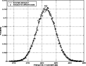
Choosing the interval in this way restricts the hidden message size to a maximum of $50\%$ of the available redundant bits. We explain in Section 6 why this is not a serious restriction. Not using all the redundant bits gives the selection process a greater opportunity to find a good embedding, as described in Section 3.3. It also leaves enough bits for the correcting transform to preserve frequency count based statistics.

Because the PRNG is keyed with a secret, it is not possible to find the hidden message without knowing the key. The recipient initializes the PRNG with that secret and uses the same selection process to retrieve the hidden message from the stego medium. The interval size is changed only after the state has been embedded, so the state is retrievable and can be used to reseed the pseudo-random number generator correctly.

Beneficial Reseeding of the PRNG

In the selection process, the keyed pseudo-random number generator can be reseeded with a freely chosen 16-bit seed. In effect, the seed creates a family of independent pseudo-random number generators. Each pseudo-random number generator selects its own subset of redundant bits. The selections result in a different number of bits that have to be modified. The distribution of the number of changed bits is binomial. The probability that k of n bits will be changed is as follows,

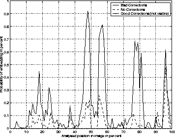
As the hidden data has been encrypted by the RC4 stream cipher, it has the properties of a random stream, so we expect that $p = \frac{1}{2}$ , and that the average number of changed bits will be close to $50\%$ of the bits in the hidden data.

Picking a seed that represents the changed bits at the lower end of the binomial distribution allows us to reduce the number of bits that have to be modified; see Figure 1. It becomes harder to detect the modifications, as more of the hidden message is already naturally represented in the redundant bits.

**Figure 1:** Probability distribution of changed bits for different seeds compared to a binomial distribution with n = 4430 and $p = \frac{1}{2}$ .
$\begin{figure} \centerline{ \epsfig {file=gauss-new.ps,width=8cm} }\end{figure}$

Detectability is also used as a bias in the selection process. The selector does not try to reduce only the number of changed bits but also the overall detectability. Whenever a bit has to be modified, its detectability will be added to a global bias. A higher accumulated bias reduces the likelihood that this specific embedding will be used.

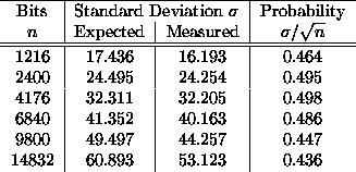
**Figure 2:** Deriving the probability p that a selected bit has to be changed from the size of a hidden message in bits n and the standard deviation $\sigma$ for embedding into a JPEG-image with 77135 redundant bits.
$\begin{figure} \begin{center} \begin{tabular} {c\vert c\vert c\vert c} \hline Bi... ...447 \ 14832 & 60.893 & 53.123 & 0.436 \ \end{tabular}\end{center}\end{figure}$

The standard deviation of a binomial distribution is given by $\sigma = \sqrt{npq}$ with q = 1 - p; in our case $\sigma = \frac{1}{2}\sqrt{n}$ . We notice that the ratio of the standard deviation and the square root of the number of bits in the hidden message remains constant,

Measuring the standard deviation of changed bits encountered in the selection step allows us to verify the probability p that a selected bit has to be modified as shown in Figure 2.

Furthermore, by varying the seed the algorithm is able to find an embedding that does not have conflicts with locked bits. This allows us to hide multiple data sets within a cover medium, which we discuss in Section 3.5.

Choices with Coding Theory

Coding theory provides us with codes that can correct errors by maximum-likelihood decoding. We write [n,k,d] to indicate a k-dimensional linear code of length n with Hamming distance d. Such a code can correct t errors, where d = 2t + 1.

In general, the application of an error-correcting code increases the data that we need to embed. A k-bit data block will result in an n-bit code block. However, we first observe that about one half of the data is already represented and does not need to be modified, and second, that we can introduce t additional errors in the code block. Thus, if

$\begin{displaymath} \frac{n}{2} - t = \frac{k}{2}\end{displaymath}$

(1)

holds, we expect the number of modifications for the encoded data to be the same as for the unencoded data. Equation (1) can be rewritten as

Unfortunately, the only non-trivial binary MDS code is the repetition code [n,1,n]. It's major drawback is the n-fold repetition of the data, so that it is useful only for small hidden messages.

Once the data is encoded, we can choose t bits in each code block that do not need to be modified in the redundant data. Our choice is determined by conflicts with already locked bits from a previously embedded message, and after all conflicts have been resolved by the detectability of changes.

The approach that we take here is similar to the parity encoding suggested by Anderson [1]. However, using error-correcting codes has advantages over using the parity encoding. We can trade security against capacity by choosing a code that is not MDS. Additionally with error-correcting codes only n-t bits are locked, whereas the parity encoding locks all n bits.

Plausible Deniability

The originator of the stego medium might now be forced to reveal the hidden communication. However, we assume that the only predicate the observer can ascertain is the fact that the cover medium was modified. If the sender embeds multiple hidden messages into the cover medium, he can include an innocuous message, turn that over on request, claim that there is no other information hidden in the stego medium, and leave unharmed. This is called plausible deniability.

Actually, the described mechanism already implicitly supports plausible deniability. More than one hidden message can be embedded, as the ``locked bit'' attribute prevents information from other hidden messages from being overwritten. Depending on the size of the hidden messages, the likelihood that a selection is found that does not conflict with previously locked bits can be small. In that case, error-correcting codes can be employed to increase the selection flexibility.

Hidden Message Determines Cover

Usually, a hidden message is embedded into a specific medium. Instead of selecting a specific cover medium, the hidden message can be examined and a cover medium will be selected that allows embedding with minimal modifications.

This can be achieved by embedding the hidden message into multiple cover media. Afterwards, the cover medium that results in the fewest modifications is chosen.

As expected, the distribution of changed bits in the different cover media follows a binomial distribution similar to the one shown in Section 3.3.

JPEG image format

The JPEG image format uses a discrete cosine transform (DCT) to transform successive $8\times8$ -pixel blocks of the image into 64 DCT coefficients each. The DCT coefficients F(u,v), of an $8\times8$ block of image pixels f(x,y), are given by

$\begin{displaymath} \begin{split} F(u,v) = \frac{1}{4}C(u)C(v) \Bigl[ \sum^7_{x=... ...+ 1)u\pi}{16}} \cos{\frac{(2y + 1)v\pi}{16}} \Bigr],\end{split}\end{displaymath}$

$\begin{displaymath} F^Q(u,v) = \text{IntegerRound}\Bigl(\frac{F(u,v)}{Q(u,v)}\Bigr),\end{displaymath}$

The least-significant bits of those quantized DCT coefficients, for which $F^Q(u,v) \not= 0$ and $\not = 1$ , are used as redundant bits into which the hidden message is embedded.

**Figure 3:** Differences in the DCT histograms are noticeable when the embedding process does not make any statistical corrections.
$\begin{figure} \centerline{ \epsfig {file=ana-normal3.ps,width=8.5cm} }\end{figure}$

Statistical Tests

The simplest test is to measure the correlation towards one. A more sophisticated one is Ueli Maurer's ``Universal Statistical Test for Random Bit Generators'' [5]. We expect images with hidden data to have a higher entropy than those without.

Westfeld and Pfitzmann outline an interesting statistical attack [13]. They observe that for a given image, the embedding of encrypted data changes the histogram of color frequencies in a particular way.

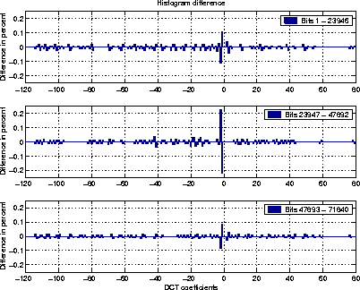
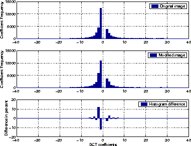
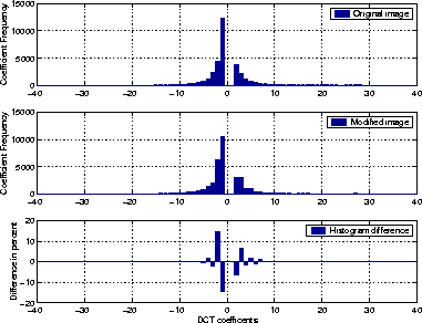
In the following, we clarify their approach and show how it applies to the JPEG format. In their case, the embedding process changes the least significant bits of the colors in an image. The colors are addressed by their indices in the color table. If n_i and $n^\ast_i$ are the frequencies of the color indices before and after the embedding respectively, then the following relation is likely to hold

$\begin{displaymath} \vert n_{2i} - n_{2i+1}\vert \geq \vert n^\ast_{2i} - n^\ast_{2i+1}\vert.\end{displaymath}$

In other words, the frequency difference between adjacent colors is reduced by the embedding process. In an encrypted message, zeros and ones are equally distributed. For n_2i > n_2i+1 that means that the bits of the hidden message change n_2i to n_2i+1 more frequently than the other way around.

The same is true in the case of the JPEG data format. Instead of measuring the color frequencies, we observe differences in the frequency of the DCT coefficients. Figure 3 displays the histogram before and after a hidden message has been embedded in a JPEG image. The histogram differences are displayed in the subgraph at the bottom of the figure. We observe a reduction in the frequency difference between coefficient -1 and its adjacent DCT coefficient -2. Adjacent means that the coefficients differ only in the least significant bit. A similar reduction in frequency difference can be observed between coefficients 2 and 3.

Westfeld and Pfitzmann use a $\chi^2$ -test to determine whether the color frequency distribution in an image matches a distribution that shows distortion from embedding hidden data. In the following, we outline their test for the DCT coefficients in a JPEG. Because the test uses only the stego medium, the expected distribution $y^\ast_i$ for the $\chi^2$ -test has to be computed from the image. The assumption for a modified image is that adjacent DCT frequencies are similar. Let n_i be the DCT histogram, we then take the arithmetic mean,

$\begin{displaymath} \chi^2 = \sum_{i=1}^{\nu+1} \frac{(y_i - y^\ast_i)^2}{y^\ast_i},\end{displaymath}$

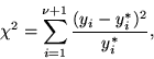
The probability p that the two distributions are equal is given by the complement of the cumulative distribution function,

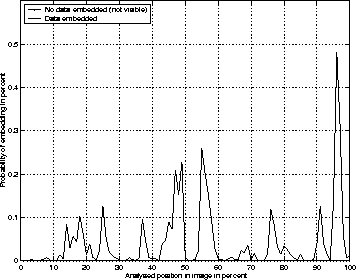
$\begin{displaymath} p = 1 - \int^{\chi^2}_0\frac{t^{(\nu-2)/2}e^{-t/2}}{2^{\nu/2}\Gamma(\nu/2)} dt,\end{displaymath}$

The probability of embedding is determined by calculating p for a sample from the DCT coefficients. The samples start at the beginning of the image and for each measurement the sample size is increased.

**Figure 4:** An extended $\chi^2$ -test where each sample covers $3.2\%$ of the DCT coefficients detects the embedding in the modified image, but does not react to an unmodified image.
$\begin{figure} \centerline{ \epsfig {file=chisqnormal2.ps,width=8cm} }\end{figure}$

Because the test uses an increasing sample size and always starts at the beginning of the image, it detects changes only if the frequency histogram is distorted continuously from the beginning of the image. Intermediate areas in the image that do not exhibit distortions can cause negative test results. This is the case even if other areas in the image are clearly distorted. For this reason, the test does not detect the embedding process described in this paper.

Detection

In this case, the sample size is set to $3.2\%$ of all DCT coefficients. The test starts at the beginning of the image, and the position is incremented by one percent for every $\chi^2$ application. This extended test does not react to an unmodified image, but detects the embedding in some areas of the stego image.

To find an appropriate sample size, we choose an expected distribution for the extended $\chi^2$ -test that should cause a negative test result. Instead of calculating the arithmetic mean of coefficients and their adjacent ones, we take the arithmetic mean of two unrelated coefficients,

A binary search on the sample size is used to find a value for which the extended $\chi^2$ -test does not show a correlation to the expected distribution derived from unrelated coefficients.

**Figure 5:** The naive statistical corrections cause the frequency of adjacent DCT coefficients to be equalized. It is immediately evident that the image is modified.
$\begin{figure} \centerline{ \epsfig {file=ana-badfoil3.ps,width=8.5cm} }\end{figure}$

Correcting Statistical Deviations

If we know what kind of statistical tests are being used to examine an image for modification, we can use the remaining redundant bits to correct any statistical deviation that the embedding process created.

Our first (naive) approach included preserving the correlation to one and the entropy measured by the Maurer test. Essentially, when a bit is changed from zero to a one, we try to change a nearby bit from one to zero. Although, this approach helps to prevent entropy increase in the redundant data, it completely neglects statistics that depend on macroscopic properties. For the JPEG format, the result is a distortion in the DCT histogram, illustrated in Figure 5. The DCT coefficients -2 and -1 are even closer together than in Figure 3, and the frequencies for DCT coefficients 2 and 3 are nearly the same.

If we want to avoid distortions in the DCT histogram, additional corrections are necessary to maintain the distribution of the DCT coefficients. For example, suppose embedding a hidden message modifies the j-th DCT coefficient, DCT(j). If DCT(j) = 2i, it will be modified to 2i+1. We correct this change by finding an adjacent coefficient DCT(k), that is DCT(k) = 2i+1, and changing it to 2i. If we correct every change to the DCT coefficients, their histogram will be identical to the one of the original image.

Furthermore, a correcting transform that essentially swaps values keeps all frequency counts constant. Thus, no statistic that is based purely on frequency counts will be able to detect a difference between the original and the stego medium.

We make the following observation for frequency count based statistics. Let f be a frequency count in the histogram, and $\bar{f}$ its adjacent count. Without loss of generality, let $f \ge \bar{f}$ . Let $\alpha$ denote the fraction of redundant bits that are used to hold the hidden message. After embedding, we expect the following changes in frequencies:

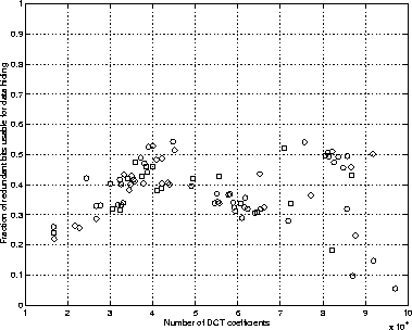
In order for the transform to be able to correct the frequency count, enough unmodified coefficients need to be left in $\bar{f}$ so that the change in f can be adjusted, in other words the relation

$\begin{displaymath} (1 - \alpha)\bar{f} \ge \frac{\alpha}{2} (f - \bar{f})\end{displaymath}$

The relation yields an a priori estimate for the fraction $\alpha$ of redundant bits that can be used for data while still having enough bits left for the correcting transform to work:

$\begin{displaymath} \alpha \le \frac{2 \bar{f}}{f + \bar{f}}.\end{displaymath}$

Given a hidden message, we can use the estimate to choose an image for which the correcting transform will be able to preserve the original frequency counts. Interestingly enough, for JPEG the fraction of redundant bits that can be used to hold the hidden message does not increase linearly for images with more DCT coefficients; see Figure 6.

**Figure 6:** The fraction of the DCT coefficients that can be used for data hiding does not increase linearly for images with more coefficients.
$\begin{figure} \centerline{ \epsfig {file=dist-use.ps,width=8.5cm} }\end{figure}$

Some statistical properties of the DCT coefficients may be unknown to us, so we try to prevent introducing additional distortions. Such distortions can result from corrections meant to preserve the statistics that we do know about. If we keep the number of additional modifications small, we reduce the likelihood of further distorting the image's statistical properties.

Furthermore, if steganography is to remain undetected by the extended $\chi^2$ -test, all parts of the image must be free of statistical distortions. The test will detect no embedding if each part of the modified image has a DCT coefficient distribution similar to the original.

$\begin{algorithm} % latex2html id marker 230 [htb] \caption{This transform prese... ... 0$} { decrement $N_{\text{error}}[i]$\; $exchDCT(k, i)$\; } }\end{algorithm}$

Algorithm 1 meets both requirements. It is run after the embedding process finishes. In step 1, we compute the DCT frequency histogram from the original image and store it in N. Step 2 determines the threshold frequencies. The threshold indicates how many errors in the histogram we are willing to tolerate for a specific DCT coefficient. It is calculated by multiplying the observed frequencies of the DCT coefficients with the scaling factor $\alpha$ . When the number of errors for a coefficient exceeds its threshold, we modify the image to preserve the statistics for that coefficient.

Step 3 finds AdjDCT, the index of the coefficient adjacent to the modified one. In step 4, we determine if there are pending errors for the adjacent coefficient that should be corrected. In that case, the correction for the current DCT coefficient can be traded against the pending correction of its adjacent coefficient.

If that is not the case, we check in step 5 if the number of errors for the coefficient, $N_{\text{error}}[DCT(i)]$ , can be incremented without exceeding its threshold value. If another increment is possible, we continue with the next modification. Otherwise, we have to correct the current modification in the image. The exchDCT algorithm is responsible for that. If that fails too, we just go ahead and increase the error for the coefficient above the threshold and take care of it later.

After all modifications have been examined, we need to correct all remaining errors. Not all the corrections might be possible. However, if we are able to correct most of the errors, changes in the histogram are not detectable.

The exchDCT() algorithm is very simple. Given a coefficient value DCT and a position i in the image, it tries to find the same coefficient at a prior position and change it to its adjacent coefficient. It starts searching near the coefficient that caused the algorithm to be executed and works its way to the beginning of the image. Coefficients that hold data from the hidden message or that have been used for previous corrections are skipped by exchDCT(). The algorithm indicates success or failure.

$\begin{algorithm} % latex2html id marker 261 [htb] \caption{Find a specific DCT ... ...DCT(j) \leftarrow AdjDCT$\; \KwRet{success} } } \KwRet{failure}\end{algorithm}$

Analysis

For this set of images, the average number of DCT coefficients that we can use for modification is about 46,000, varying between 30,000 and 97,000. Each of these contributes one redundant bit.

Without embedding any data in the redundant bits, we notice a strong correlation towards one. On average, $63.8\%$ of all the bits are set with a standard deviation of $\pm 3.4\%$ between images.

We embedded the first chapter of Lewis Carroll's ``The Hunting of the Snark'' into the images. After compression, the hidden message had a size of about 14,700 bits.

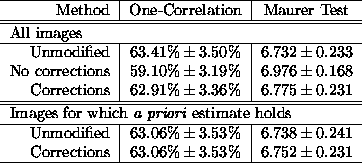
**Figure 7:** Comparison between unmodified images, images with data embedded but without statistical corrections, and finally images with data embedded plus statistical corrections.
$\begin{figure} \begin{center} \begin{tabular} {r\vert c\vert c} \hline Method & ... ...$\space & $6.752 \pm 0.231$\space \ \hline\end{tabular}\end{center}\end{figure}$

Figure 7 shows the results for the simple statistics that operate only on the redundant data. With a block size of eight bits, the result of the Maurer test for a truly random source is 7.184. We observe a noticeable increase in entropy for images that have not received statistical correction. The correlation towards one decreases noticeably, too. However, for the images that have been corrected for statistical distortions the values are very close to the data from the unmodified images. Examining only the images for which the a priori estimate holds, we notice that the differences between the unmodified images and the images that received corrections are even smaller. These simple tests are thus not able to detect our steganography.

**Figure 8:** The extended $\chi^2$ -test detects the embedding for the image that has no statistical corrections. Our naive correction is even more detectable. However, an image that receives the proper statistical correction can not be distinguished from an unmodified image.
$\begin{figure} \centerline{ \epsfig {file=chisquare3.ps,width=8cm} }\end{figure}$

The more interesting statistic is the DCT frequency histogram. If we plot the DCT histogram of images that have received corrections, we are no longer able to find noticeable differences in the distribution. Figure 8 shows the extended $\chi^2$ -test. The test detects the image without corrections and the image corrected with our naive method, but it is unable to detect the image corrected for statistical deviations with the transform in Algorithm 1.

The correcting transform causes about $2967 \pm 434$ additional changes to the redundant data. That is approximately $20\%$ of the size of the hidden message. The average number of differences that can not be corrected is $186 \pm 400$ . The majority of corrections fail for images for which the a priori estimate indicates a maximum message size that was smaller than the one we try to embed. However, if we look only at images for which the estimate holds, the correcting transform changes $3106 \pm 415$ bits and the average number of differences that can not be corrected is $5 \pm 5.7$ .

It is possible to further decrease the changes from the correcting transform, by biasing the selection algorithm against modifying coefficients with a higher frequency than their adjacent coefficients. The identification step from Section 3.1 adds the annotation that changes to bits originating from higher frequency coefficients are easier to detect. Using the worst selection, the correcting transform causes $3365 \pm 442$ additional changes. The best selection results in only $3054 \pm 430$ changes. Comparing each image, we see that using this technique, the correcting transform can avoid $311 \pm 68$ changes in average.

To verify the correctness of the a priori estimate, we embed messages of different sizes and apply the correcting transform. We note that for message sizes below the estimate the transform is able to correct most errors. Increasing the message size above the estimate causes a noticeable increase in errors.

**Figure 9:** Examining the differences in the DCT histogram for parts of the image shows no noticeable deviations from the unmodified original. The largest difference is around $0.2\%$ .
$\begin{figure} \centerline{ \epsfig {file=ana-histinparts-5.ps,width=9cm} }\end{figure}$

The transform also has to meet the restriction that there be no area in the image that shows noticeable distortion in the DCT coefficients. Figure 9 shows the histogram difference of a modified image in comparison to the original. The differences in the frequency of the DCT coefficients are negligible, thus the extended $\chi^2$ -test does not indicate any hidden data.

Conclusion

We introduced two new methods to improve the selection process. The first uses a seeded pseudo-random number generator to determine the fewest modifications to the cover medium. The second uses error-correcting codes to increase the flexibility in selecting bits without increasing the number of necessary changes. Together, these methods can be used to provide plausible deniability be embedding multiple hidden messages in the cover medium.

Although the commonly used $\chi^2$ -test is unable to detect modifications from the improved embedding process described in this paper, we described an extended $\chi^2$ -test that is capable of detecting modified areas in parts of an image.

To counter statistical tests based on frequency counts like the extended $\chi^2$ -test, we introduced a new method to correct the statistical deviations from the embedding process and a correcting transform for the JPEG format. As a result, none of the presented statistical tests can detect the presence of steganography. We also presented an a priori estimate that allows us to determine the amount of data that can be hidden in an image while still being able to preserve frequency count based statistics. Given a hidden message, we can use the estimate to quickly choose an image in which a specific message can be embedded safely.

The methods to improve the embedding and to apply correcting transforms to preserve statistical properties have been implemented in the OutGuess [8] program, which is freely available as source code at www.outguess.org.

Acknowledgments

References

About this document ...

This document was generated using the LaTeX2HTML translator Version 97.1 (release) (July 13th, 1997)

Defending Against Statistical Steganalysis

References

About this document ...Defending Against Statistical SteganalysisThis document was generated using the LaTeX2HTML translator Version 97.1 (release) (July 13th, 1997) Copyright © 1993, 1994, 1995, 1996, 1997, Nikos Drakos, Computer Based Learning Unit, University of Leeds.
The command line arguments were:
The translation was initiated by Charlie & on 5/10/2001 Footnotes
Charlie & 5/10/2001 |