| ||||||||||||||||||||||||||||||||||||||||||||||||||||
|
OSDI '04 Paper
[OSDI '04 Technical Program]
PlanetSeer: Internet Path Failure Monitoring
|
|
We divide the ProbeD nodes into 30 groups based on geographic diversity, as shown in Table 1, mainly to reduce the number of probes launched per anomaly. Probing every anomaly from every ProbeD location would yield too much traffic (especially to sites with conservative intrusion detection systems), and the extra traffic may not yield much insight if many nodes share the same paths to the anomaly. We also divide North America into educational and non-educational groups, because the educational (.edu) sites are mostly connected to Internet2, while non-educational sites are mostly connected by commercial ISPs.
When a ProbeD receives a request from its local MonD, it forwards it to a ProbeD in each of the other groups. The ProbeDs perform the forward probes, and send the results back to the requester. All results are collected by the originator, and logged with other details, such as remote IP address and the current time.
We have been running PlanetSeer since February 2004. In three months, we have seen 887,521 unique clients IPs, coming from 9232 Autonomous Systems (ASes) (according to previous IP-to-AS mappings techniques [17]). Our probes have traversed 10090 ASes, well over half of all ASes on the Internet. We use a hierarchical AS classification scheme that has five tiers, based on AS relationships and connectivity [23]. The highest layer (tier 1) represents the dense core of the Internet, and consists of 22 ASes of the largest ISPs. Tier 2 typically includes ASes of other large national ISPs. Tier 3 includes ASes of regional ISPs. Finally, tiers 4 and 5 include ASes of small regional ISPs and customer ASes respectively. As shown in Table 2, we have very good coverage of the top 4 AS tiers, with complete coverage of tier 1 and nearly-complete coverage of tier 2.
|
Having collected the passive data from MonD and the traceroutes from ProbeD, the next step is processing the probes to confirm the existence of the anomaly. This section describes how we use this data to classify anomalies and quantify their scope. It also reports how different types of anomalies influence end-to-end performance.
Some of the data we receive from the traceroutes is incomplete or unusable, but we can often perform some simple processing on it to salvage it. The unusable hops in a traceroute are those that do not identify the routers or that identify the routers by special-use IP addressess [11]. The missing data is generally the absence of a hop, and can be interpolated from other traceroutes.
Identifying and pruning unusable hops in traceroute is simple: the unusable hops are identified by asterisks in place of names, and other than showing the existence of these hops, these data items provide no useful information. We simply remove them from the traceroute but keep the relative hop count difference between the existing hops.
Missing hops in a traceroute are slightly harder to detect, but we
can
use overlapping portions of multiple traceroutes to infer where they
occur. We use a simple heuristic to identify the missing hops: we
compare traceroutes that share the same destination, and if the hops
leading to the destination differ by an intermediate hop that is
present in one and missing in the other, we replace the missing hop
with the address in the other trace. Put more formally, given two
traceroutes from two sources to the same destination, suppose there
are two subsequences of these two traceroutes, ![]() and
and ![]() (
(![]() and
and ![]() ) such
that
) such
that ![]() and
and ![]() . We define
. We define ![]() to be the hop count of
to be the hop count of
![]() . Note that the number of hops between
. Note that the number of hops between ![]() and
and ![]() ,
, ![]() , can be greater than
, can be greater than ![]() , because we have
removed ``*''
and special-use IPs from the traceroutes. If
, because we have
removed ``*''
and special-use IPs from the traceroutes. If ![]() , it is very likely
that all the hops in
, it is very likely
that all the hops in ![]() and
and ![]() are the same since they merge at
are the same since they merge at ![]() (
(![]() ) and follow the
same number of hops to
) and follow the
same number of hops to ![]() (
(![]() ). If there exists
). If there exists ![]() such that
the hop corresponds to
such that
the hop corresponds to ![]() in
in ![]() does
not exist because it has been removed as ``*'', we consider
does
not exist because it has been removed as ``*'', we consider ![]() a
missing hop in
a
missing hop in ![]() and add this hop into
and add this hop into ![]() .
.
Our approach to inserting missing hops helps us filter out the
``noise'' in traceroutes so that it does not confuse our anomaly
confirmation using route change as described in
Section 4.2. However, it may mask
certain hop
differences. For example, we sometimes see two paths ![]() and
and ![]() merge
at
merge
at ![]() (
(![]() ), and diverge at some later hops
before merging at
), and diverge at some later hops
before merging at
![]() (
(![]() ) again. This usually occurs between
tightly-coupled
routers for load balancing reasons, where a router selects the next
hop from several parallel links based on the packet IP addresses
and/or traffic load [19]. In
this case, inserting missing
hops may eliminate the different hops between the two traceroutes.
) again. This usually occurs between
tightly-coupled
routers for load balancing reasons, where a router selects the next
hop from several parallel links based on the packet IP addresses
and/or traffic load [19]. In
this case, inserting missing
hops may eliminate the different hops between the two traceroutes.
For our purposes, we do not treat such ``fluttering'' [19]
as anomalies because it occurs as a normal practice. We detect
fluttering by looking for hops ![]() and
and ![]() such that
such that ![]() but
but ![]() , and we merge them
into the same hop in all the traceroutes. Note that this could also
possibly eliminate the hop difference caused by path change and lead
to underestimating the number of anomalies.
, and we merge them
into the same hop in all the traceroutes. Note that this could also
possibly eliminate the hop difference caused by path change and lead
to underestimating the number of anomalies.
|
After we have processed the traceroutes, we are ready to decide whether an event reported by MonD is actually an anomaly. We consider an anomaly ``confirmed'' if any of the following conditions is met:
Our confirmation process is very conservative--it is possible that some of the reported anomalies are real, but do not meet any of the above conditions. However, our goal is to obtain enough samples of anomalies for our analysis and we do not want our results to be tainted by false positives. Hence, we choose stricter conditions for confirming anomalies. Similarly, we confirm a reported anomaly as non-anomaly if the local traceroute does not contain any loop, agrees with the baseline traceroute, and reaches the destination. For a confirmed non-anomaly, we do not perform traceroutes at remote ProbeDs, in order to reduce measurement traffic.
|
In three months, we have seen a total of 2,259,588 possible anomalies reported, of which we confirmed 271,898. Table 3 shows the number of reported anomalies of each type. As we can see, TTL change is the most common type of reported anomaly, accounting for 44% of the reported anomalies. For the remaining anomalies triggered by timeouts, passive monitoring suggests that 23% are most likely caused by forward path problems.
Table 4 shows the breakdown
of anomalies using
the 4 confirmation conditions. The non-anomalies account for 2/3 of the
reported anomalies. Among the
possible reasons for the occurrence of non-anomalies are: ultrashort
anomalies, path-based TTL, and aggressive consecutive timeout levels.
Some anomalies, which we term ultrashort, are so short that our system
is unable to respond in time. Since they often are in the process of
being resolved when the forward probes are taking place, the
traceroute results may be inconsistent.
Many false alarms from path-based TTL changes are due to NAT
boxes. When clients with different initial TTL values share a NAT
box, their interleaved packets appear to show TTL change. Using
flow-based TTL change would reduce these false alarms, but may miss
real TTL changes that occur between flows since any path history would
be lost. Finally, our consecutive timeout conditions may be
aggressive for hosts with short timeout periods. Excluding the
non-anomalies, we confirm 271898 (35%) of the remaining anomalies and
probe them from multiple vantage points. We use these anomalies for
our analysis in the remainder of this paper.
|
This section focuses on analyzing routing loops, which can occur due to inconsistencies in routing state, misconfiguration, and other causes. We are interested in their frequency, duration, size, location, and effect on end-to-end performance.
We detect routing loops by observing the same sequence of routers appearing several times in a traceroute. Since loops in traceroute may reflect upstream routing changes rather than true routing loops [19], we choose to take a conservative approach and require that the same sequence appear in a traceroute at least 3 times before we confirm it as a routing loop.
Using this metric, we identify a total number of 21565 routing loops in our data. If we relax the loop condition to allow loops that have the same sequence only twice, this count increases to 119,936, almost six times as many. Using this approach, our overall confirmed anomaly count would increase 36% to over 370K.
Loops are separated into persistent and temporary loops [19] based on whether the traceroute was ultimately able to exit the loop. If the traceroute stays within the loop until the maximum number of hops (32 in our case), we classify it as persistent, while if the loop is resolved before the traceroute reaches the maximum hop, it is temporary. Temporary loops can occur due to the time necessary to propagate updated routing information to the different parts of the network, while persistent loops can be caused by various reasons, including router misconfiguration [16]. Persistent loops tend to last longer and may require human intervention to be resolved, so they are considered more harmful. About 83% of the observed loops are persistent, as shown in Table 5. Since temporary loops only exist for a short period, it may be harder to catch them.
We use the reprobes to determine duration of the persistent loops. The reprobes for some persistent loops are missing, often because the local PlanetLab node failed or rebooted before all reprobes completed. For those loops, we do not know when the loops were resolved. We only include the loops having all 4 reprobes in our analysis. Therefore, we show the percentage of loops in each duration instead of the exact numbers in Table 5. We can see many persistent loops are either resolved quickly (54% terminate within half an hour) or last for a long time (23% stay for more than 7.5 hours).
Previous research has noted that routing loops are likely to be correlated [19], because nearby routers usually share routing information very quickly. If some routers have inconsistent information, such information is likely to be propagated to other nearby routers and cause those routers to form loops. We observe a similar phenomenon, which is quantified in Table 5. We count the number of distinct loops in traceroutes from other ProbeDs during the same period. We find that 16% of the temporary loops are accompanied by at least one disjoint loop while only 6% of the persistent loops see them. We suspect the reason is temporary loops are more likely to stem from inconsistent routing state while persistent loops are more likely to be caused by other factors which may not be related to routing inconsistency.
Finally, using the persistent loop data, we can also get some insight into the relative distribution of AS quality by measuring how evenly-distributed the loops are. Since these loops are largely single-AS, they are very unlikely to arise from external factors, and may provide some insight into the monitoring/management quality of the AS operators. We use a metric, which we call skew, to provide some insight into the distribution. We calculate skew as the percentage of per-tier loops seen by the ``worst'' 10% of the ASes in that tier. A skew value of 10% indicates all ASes in the tier are likely to be uniform in the quality, while larger numbers indicate a wider disparity between the best ASes and the worst.
In tier 1, the top 2 ASes (10% of 22) account for 35% of the loops, while in tier 2, the top 21 ASes (10% of 215) account for 97% of the loops. This skew may translate into different reliabilities for the customers they serve. The disparity in traffic must also be considered when judging how important these skew numbers are. With respect to the traffic that we observe, we find that these ASes account for 20% of tier 1 traffic and 63% of tier 2 traffic. The disparity between the loop rates and the traffic for these ASes would indicate that these ASes appear to be much more problematic than others in their tier.
Besides their frequency, one of the other factors that determines the effect of routing loops is their scope, including how many routers/ASes are involved in the loop, and where they are located. We use the term loop length to refer to the number of routers involved, and we show a breakdown of this metric in Table 6. The most noticeable feature is that temporary loops have much longer lengths than persistent loops. 97% of the persistent loops consist of only 2 routers, while the ratio is only 50% for temporary loops. Intuitively, the more routers are involved in a loop, the less stable it is. Therefore, most persistent loops exist between only two routers, while temporary loops span additional routers as the inconsistent state propagates.
We next examine the number of ASes that are involved in the loops. The breakdown is shown in Table 5, which shows that persistent loops overwhelmingly occur within a single AS, while 15% of temporary loops span multiple ASes. Ideally, BGP prevents any inter-AS loops by prohibiting a router from accepting an AS path with its own AS number in that path. However, BGP allows transient inconsistency, which can arise during route withdrawals and announcements [10], and this is why we see more temporary loops spanning multiple ASes. In contrast, persistent loops can occur due to static routing [19] or router misconfigurations [16]. Given how few persistent loops span multiple ASes, it appears that BGP's loop suppression mechanism is effective.
To understand where loops arise, we classify them according to the hierarchy of ASes involved. In theory, we could calculate their depth [7], which would tell us the minimum number of hops from the routers to the network edge. However, since we cannot launch probes from the clients, this depth metric would be misleading. If the loop occurs on an AS that does not lie near any of our ProbeD locations, our probes travel through the network core to reach it, and we would believe it to be very far from the edge. If we could launch probes from the clients, network depth would be meaningful.
We map loops into tiers by using the tier(s) of the AS(es) involved. A loop can be mapped to multiple tiers if it involves multiple ASes. Table 5 shows the number of loops occurring in each tier. Tier-1 and tier-2 ASes have very few persistent loops, possibly because they are better provisioned than smaller ASes. A large portion of loops (40% for temporary and 46% for persistent) occur in tier-3 (outer core) ASes, which suggests that the paths in those large regional ASes are less stable. In Table 6, we compare the loops in the core network (tiers 1, 2, 3) or the edge network (tiers 4, 5). As the table shows, both temporary and persistent loops are likely to involve more hops if occurring in the core network.
Loops can degrade end-to-end performance in two ways: by overloading routers due to processing the same packet multiple times [10] (for temporary loops), or by leading to loss of connectivity between pairs of hosts (for permanent loops). Since MonD monitors all flows between the node and remote hosts, we can use the network statistics it keeps to understand end-to-end effects.
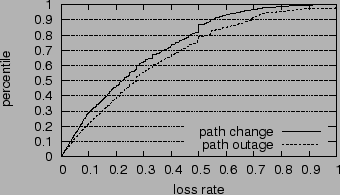
When MonD suspects an anomaly, it logs the retransmission rate and RTT leading up to that point. Retransmission rates are calculated for the last 5 minutes. RTTs are calculated using an Exponentially Weighted Moving Average (EWMA) with the most recent value given a weight of 1/8, similar to that used in TCP. Figure 1 shows the CDF of the retransmission rate, and we see that 65% of the temporary loops and 55% of the persistent loops are preceded by loss rates exceeding 30%. Since the typical Internet loss rate is less than 5% [20], this higher loss rate will significantly reduce end-user TCP performance prior to the start of the anomaly.
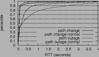
In addition to the high loss rates, loop anomalies are also preceded by high latency, as shown in Figure 2. High latency can be caused by queuing due to congestion or packets repeatedly traversing the same sequence of routers. We compare the RTT right before loops occur with the RTT measured in the baseline traceroute on the same path. It is evident that loops can significantly degrade RTTs.
While loop-based anomalies are relatively simple to identify, they represent a relatively small fraction of the total confirmed anomalies. Classifying the other anomalies, however, requires more effort. This section discusses the steps taken to classify the non-loop anomalies, and the complications involved. The main problem is how to determine that the anomaly occurs on the forward path from the local node to the destination. Additionally, we want to characterize the anomaly's features, such as its pattern, location and affected routers.
To deal with these two problems, we need a reference path from the local node to the destination, which represents the path before the anomaly occurs. Then we can compare it against the local traceroute during the anomaly. This comparison serves three purposes: First, it can help us distinguish between forward-path and reverse-path anomalies. If the local path during the anomaly is different from the reference path, the route change usually indicates that the anomaly is on the forward path. Second, it can be used to quantify the scope of the anomaly. By examining which routers overlap between the local path and the reference path, we can estimate which routers are potentially affected by the anomaly. It can also be used to determine the location of the anomaly, in terms of the number of the router hops between the anomaly and the end hosts. Third, it is used to classify the anomalies. Based on whether the local traceroute reaches the last hop of the reference path, we can classify it as either path change or path outage.
Ideally, we could simply use the baseline traceroute as the reference path, if it successfully reaches the destination. If the local traceroute during an anomaly stops at some intermediate hop, we know it is an outage. If the local traceroute is different, but reaches the destination, we know it is a routing change. However, the baseline traceroute may not reach the destination for a variety reasons. Some of these include:
The rest of this section focuses on deciding whether the baseline
traceroute can be used as the reference path when it does not reach
the destination. If a baseline path ![]() stops at hop
stops at hop ![]() , we try to guess if
, we try to guess if ![]() is a firewall using some heuristics.
is a firewall using some heuristics. ![]() must meet the
following
four requirements before we consider it a firewall:
must meet the
following
four requirements before we consider it a firewall:
The first three requirements are easy to verify, so we focus
on the last requirement. Let ![]() be the number of
hops from
hop
be the number of
hops from
hop ![]() to the local node on the reverse path. We
first want to check
if
to the local node on the reverse path. We
first want to check
if ![]() . From MonD, we know
. From MonD, we know
![]() , the TTL of a packet when it arrives at the
local node
from the destination. If the TTL is initialized to
, the TTL of a packet when it arrives at the
local node
from the destination. If the TTL is initialized to ![]() by
the destination, we have
by
the destination, we have ![]() because the TTL is decremented at each hop along the reverse path. The
issue is how to determine
because the TTL is decremented at each hop along the reverse path. The
issue is how to determine ![]() . The initial TTL
values
differ by OS, but are generally one of the following: 32 (Win
95/98/ME), 64 (Linux, Tru64), 128 (Win NT/2000/XP), or 255
(Solaris). Because most Internet paths have less than 32 hops, we can
simply try these 4 possible initial TTL values and see which one, when
subtracted by
. The initial TTL
values
differ by OS, but are generally one of the following: 32 (Win
95/98/ME), 64 (Linux, Tru64), 128 (Win NT/2000/XP), or 255
(Solaris). Because most Internet paths have less than 32 hops, we can
simply try these 4 possible initial TTL values and see which one, when
subtracted by ![]() , gives a
, gives a ![]() that is less than 32 hops. We will use that as
that is less than 32 hops. We will use that as ![]() to calculate
to calculate ![]() . Similarly, from the traceroute, we
can also calculate
. Similarly, from the traceroute, we
can also calculate ![]() using
using ![]() .
.
Although inter-AS routing can be asymmetric, intra-AS paths are
usually symmetric [19]. Since ![]() and the destination are
in the same AS, their forward hop count difference should be the same
as
their reverse hop count difference, which we are able compute as
described above.
and the destination are
in the same AS, their forward hop count difference should be the same
as
their reverse hop count difference, which we are able compute as
described above.
Choosing an appropriate ![]() for all settings is difficult, as
there
may be one or more hops between a firewall and its protected hosts.
We conservatively choose
for all settings is difficult, as
there
may be one or more hops between a firewall and its protected hosts.
We conservatively choose ![]() , which means we
consider
, which means we
consider ![]() as a valid
reference path only when
as a valid
reference path only when ![]() is one hop away from
the destination.
This will minimize the possibility that a real path outage is
interpreted as a traceroute being blocked by a firewall. However, it
leads to bias against large organizations, where end hosts are
multiple hops behind a firewall. In such cases, we cannot determine if
the anomalies are due to path outage or blocking at a firewall.
Therefore, we do not further analyze these anomalies.
is one hop away from
the destination.
This will minimize the possibility that a real path outage is
interpreted as a traceroute being blocked by a firewall. However, it
leads to bias against large organizations, where end hosts are
multiple hops behind a firewall. In such cases, we cannot determine if
the anomalies are due to path outage or blocking at a firewall.
Therefore, we do not further analyze these anomalies.
|
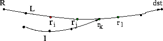
In this section, we discuss classifying anomalies by comparing the
reference path ![]() with the local path
with the local path ![]() . There are
three
possibilities when we compare
. There are
three
possibilities when we compare ![]() and
and ![]() :
:
We observe a total of 250333 non-loop anomalies, with their breakdown shown in Table 7. About half of them are path changes, and 10% are forward path outages. For the 24% that are classified as other outages, we cannot infer whether they are on the forward or reverse paths. The remaining 18% are temporary anomalies. In these cases, the first local traceroute does not match the reference path, but the second local traceroute matches. In these cases, the recovery has taken place before we can gather the results of the remote probes, making characterization impossible. While it is possible that some remote probes may see the anomaly, the rapidly-changing state is sure to cause inconsistencies if we were to analyze them. To be conservative, we do not perform any further analysis of these anomalies, and focus only on path changes and forward outages. These temporary anomalies are different from the ultrashort anomalies in that the ultrashort anomalies were already in the repair process during the first probe. So, while we choose not to analyze temporary anomalies further, we can at least inarguably confirm their existence, which is not the case with the ultrashort anomalies.
We first consider path changes, in which the local path ![]() diverges
from the reference path
diverges
from the reference path ![]() after some hops, then merges back
into
after some hops, then merges back
into ![]() and successfully terminates at the last hop of
and successfully terminates at the last hop of ![]() . This kind
of
anomaly is shown in Figure 3.
. This kind
of
anomaly is shown in Figure 3.
 |
 |
As discussed in Section 2, it is
usually very
difficult to locate the origin of path anomalies purely from
end-to-end measurement [8].
However, even if the precise
origin cannot be determined, we may be able to narrow the scope
of the anomaly. We define the scope of a path change as the
number of hops on ![]() which possibly change their next
hop
value. Flows through these routers may all have their paths
changed. In Figure 3,
which possibly change their next
hop
value. Flows through these routers may all have their paths
changed. In Figure 3, ![]() diverges from
diverges from ![]() at
at
![]() and merges into
and merges into ![]() at
at ![]() . All the hops before
. All the hops before ![]() or after
or after
![]() (including
(including ![]() ) follow the same next hop towards
the
destination. So the hops which are possibly influenced by the path
change and have different next hops are
) follow the same next hop towards
the
destination. So the hops which are possibly influenced by the path
change and have different next hops are ![]() ,
, ![]() and
and ![]() .
.
In some cases, we may be able to use remote traceroutes to narrow
the
scope even further. For example, in Figure 3, if ![]() , a traceroute
from another ProbeD merges into
, a traceroute
from another ProbeD merges into ![]() at
at ![]() , a hop that is before
, a hop that is before
![]() , we can eliminate
, we can eliminate ![]() from the scope of
the path change anomaly, since we know
from the scope of
the path change anomaly, since we know ![]() has the same next
hop value as it did in the reference path. We call
has the same next
hop value as it did in the reference path. We call ![]() the intercept
path. This method may still overestimate the scope of path change:
it is possible, for
example, that
the intercept
path. This method may still overestimate the scope of path change:
it is possible, for
example, that ![]() 's next hop value is unaffected, but
we cannot know this unless some traceroute merges into
's next hop value is unaffected, but
we cannot know this unless some traceroute merges into ![]() at
at ![]() .
.
Performing traceroute from multiple geographically diverse vantage points increases our chances of finding an intercept path. Our ability of narrowing the scope is affected by the location of the anomaly. If it is closer to the destination, we have a better chance of obtaining intercept paths by launching many forward traceroutes, and thus successfully reducing the scope of the anomaly. In contrast, if the anomaly is nearer our source, the chance of another traceroute merging into the reference path early is low.
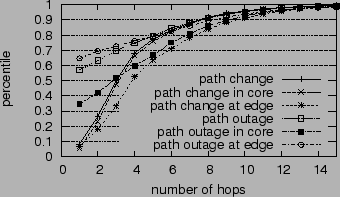
Figure 4 shows the CDF of path change scope, measured in hop count. We can confine the scope of 68% of the path changes to within 4 hops. We do not count fluttering as path changes, since these would appear as a large number of path change anomalies, each with a very small scope. We also examine how many ASes the path change scope spans, shown in Table 8. Again, we can confine the scope of 57% of the path changes to within two ASes and 82% of them to within three ASes.
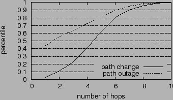
To gain some insight into the location of the anomalies, we also study whether the path change occurs near end hosts or in the middle of the path [7]. We measure the distance of a path change to the end host by averaging the distances of all the routers within the path change scope. The distance of a router is defined as the minimum number of hops to either the source or the destination. Figure 5 plots the CDF of path change distances. As we can see, 60% of the path changes occur within 5 hops to the end hosts.
We can also use AS tiers to characterize network locations, so we map the routers within anomaly scopes to ASes and AS tiers. The breakdown of possibly affected routers by their AS tiers is shown in Table 8. The routers in Tier-3 are most likely to be affected by path changes, since they account for nearly half of the total. By comparison, the routers in tier-1 ASes are rather stable, though presumably they are traversed repeatedly by many paths.
|
In Figure 4, we see that path changes in the core network have narrower scope than those in the edge. This is probably because the paths in the core network are likely to be traversed by traceroutes from many vantage points to reach the destination. In contrast, if a route change occurs near a local node, we have less chance of finding an intercept path that happens to merge into the reference path early. As a result, the anomaly scope in these cases is more loosely confined.
Since path change is a dynamic process and anomaly scopes may evolve over time, a measured anomaly scope should be viewed as a snapshot of which routers are affected when the traceroutes reach them. In Table 8, we show how many path changes have changed scope between the first and second sets of forward probes. We find that only 4% of them have changed during that period (mostly within one minute). In addition, 66% of the scope changes are due to local path changes instead of intercept path changes.
We now examine the effect of path changes on end-to-end performance. The effect of path changes on RTTs is relatively mild, as can be seen in Figures 8. The RTTs measured during path changes are only slightly worse than the RTTs measured in baseline traceroutes. But the loss rates during path changes can be very high. Nearly 45% of the path changes cause loss rates higher than 30%, which can significantly degrade TCP throughput.
We now focus on path outages and describe how to distinguish between
forward and reverse path outages. In Figure 6,
the local path ![]() stops at
stops at ![]() , which is an
intermediate hop on
the reference path
, which is an
intermediate hop on
the reference path ![]() . At first glance, one might
conclude that a
failure has occurred after
. At first glance, one might
conclude that a
failure has occurred after ![]() on the forward path,
which prevents
the packets from going through; but other possibilities also
exist--because Internet paths could be asymmetric, a failure on the
reverse path may produce the same results. For example, if a shared
link on the reverse paths from all the hops beyond
on the forward path,
which prevents
the packets from going through; but other possibilities also
exist--because Internet paths could be asymmetric, a failure on the
reverse path may produce the same results. For example, if a shared
link on the reverse paths from all the hops beyond ![]() to the
source
has failed, none of the ICMP packets from those hops can return.
Consequently, we will not see the hops after
to the
source
has failed, none of the ICMP packets from those hops can return.
Consequently, we will not see the hops after ![]() .
.
If we have control of the destination, we can simply distinguish between forward and reverse path outages using ping [7]. However, since our clients are outside of PlanetLab and not under our control, we cannot perform pings in both directions, and must use other information to disambiguate forward path outages from reverse path failures. Specifically, we can infer that the outage is on the forward path using the following rules:
Table 9 shows the number of forward path outages inferred from each rule. As we can see, all three rules are useful in identifying forward outages. More than half of the outages are accompanied by route changes, as the failure information is propagated and some routers try to bypass the failure using other routes. Forward timeouts help us infer one third of the forward outages. This demonstrates the benefit of combining passive monitoring with active probing, since we would not have been able to disambiguate them otherwise.
|
To characterize the scope of path outages, we use a technique similar
to the one we used to characterize the scope of path change. We define
a path outage scope as the number of hops in a path that cannot forward
packets to their next hop towards the destination. In
Figure 6, ![]() is the
reference path and
is the
reference path and ![]() is the local path.
is the local path. ![]() stops at
stops at ![]() , which is an
intermediate hop of
, which is an
intermediate hop of ![]() . Hence, all the hops after
. Hence, all the hops after ![]() (including
(including
![]() ) are possibly influenced by the outage and may not be able
to forward
packets to the next hops towards the destination. However, when we can
find another intercept path, we can narrow the scope.
For example, if
) are possibly influenced by the outage and may not be able
to forward
packets to the next hops towards the destination. However, when we can
find another intercept path, we can narrow the scope.
For example, if ![]() merges into
merges into ![]() at
at ![]() and reaches the destination, then only
and reaches the destination, then only ![]() and
and ![]() can possibly be influenced by the
outage. Again, this method might overestimate the scope of a path
outage, for the same reasons described earlier on estimating a path
change scope.
can possibly be influenced by the
outage. Again, this method might overestimate the scope of a path
outage, for the same reasons described earlier on estimating a path
change scope.
Note that unlike in previous work [6,7], we use a set of routers to quantify the effect of path outages instead of just using the last hop where the traceroute stops. Since outage information is usually propagated to many routers, using only one router does not give us a sense of how many routers may have been affected by the outage.
In some cases, we may not have a complete baseline path which reaches the destination or the penultimate router. In these cases, we can not estimate the scope of the forward outage because we do not know the exact number of hops between the last hop of the baseline path and the destination. We only know that the anomaly occurs somewhere on the forward path. Among all the outages, about 47% have no complete reference path. In the following, we use only those with complete reference paths in the scope analysis.
In Figure 4, we plot the CDF of the number of hops in the forward outage scope. Compared with path change, we can confine the outage scope more tightly. Nearly 60% of the outages can be confined to within 1 hop and 75% of them can be confined to 4 hops.
We suspect that such tight confinement is due to last hop failures. In Figure 5, we plot the distances of forward outages to the end hosts. The distance of an outage is defined as the average distance of the routers within the outage scope to the end hosts, similar to the definition used for path change in Section 7.1. As we can see, 44% of the outages do occur at the last hop, allowing us to confine their scopes to 1 hop. This observation explains why the outages in the edge network are confined more tightly than those in core networks, as shown in Figure 4.
Excluding last hop failures, we can only confine 14% of the outages to one hop, a result that is slightly better than that for path changes. In general, the scopes of path outages tend to be smaller than those of path changes. Compared with path changes in Figure 5, path outages tend to occur much closer to the end hosts. More than 70% of the outages occur within 4 hops to the end hosts.
Table 8 gives the number of ASes that the outages span. Compared with path changes, we can confine a much higher percentage of outages (78%) within two ASes. If we examine the AS tiers where the affected routers are located, outages are spread out more evenly across tiers than path changes are. Paths in tier-1 ASes are the most stable and those in tier-3 ASes are most unstable. If we look at both Table 5 and Table 8, we note that paths in tier-3 ASes are most likely to be affected by all types of anomalies. They account for 40% of temporary loops, 46% of persistent loops, 47% of path changes and 26% of forward outages. In contrast, paths in tier-1 ASes are most stable.
Finally, in Table 8, we find that the scopes of 10% of the forward outages might have changed between the first and second set of forward probes, mostly due to local path changes. Another 8% of the forward outages have reference paths that do not terminate at the destinations. These last hops are considered firewalls based on the heuristic described in Section 6.
We also study how path outages influence end-to-end performance. Not surprisingly, forward outages can be preceded by very high loss rates, which are slightly worse than those generated by path changes. The comparisons are shown in Figure 7. Similarly, outages tend to be preceded by much worse RTTs than path changes, as shown in Figure 8: 23% of the outages experience RTTs that are over one second, while only 7% do when there is no outage. The RTT variances can also be very high: 17% of them exceed 0.5 seconds.
In addition to characterizing anomalies, one of the goals of PlanetSeer is to provide benefits to the hosts running it. One possible approach is using the wide-area service nodes as an overlay, to bypass path failures. Existing systems, such as RON [1], bypass path failures by indirectly routing through intermediate nodes before reaching the destinations. Their published results show that around 50% of the failures on a 31-node testbed can be bypassed [7]. PlanetSeer differs in size and scope, since we are interested in serving thousands of clients that are not participants in the overlay, and we have a much higher AS-level coverage.
Determining how many failures can be bypassed in our model is more complicated, since we have no control over the clients. Clients that are behind firewalls and filter pings and traceroutes may be reachable from other overlay nodes, but we may not be able to confirm this scenario. As a result, we focus only on those destinations that are reachable in the baseline probes, since we can confirm their reachability during normal operation.
For this group of clients, we have a total of 62815 reachability failures, due to anomalies like path outages or loops. Of these failures, we find that some nodes in PlanetSeer are able to reach the destinations in 27263 cases, indicating that one-hop indirection is effective in finding a bypass path for 43% of the failures.
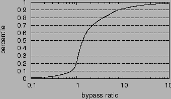
In addition to improving the reachability of clients using overlay paths, the other issue is their relative performance during failures. We calculate a bypass ratio as the ratio between the minimum RTT of any of the bypass paths and the RTT of the baseline path. These results are shown in Figure 9, and we see that the results are moderately promising - 68% of the bypass paths suffer less than a factor of two in increased latency. In fact, 23% of the new paths actually see a latency improvement, suggesting that the overlay could be used for improving route performance in addition to failure resiliency. However, some paths see much worse latency degradation, with the worst 5% seeing more than a factor of 18 worse latency. While these paths may bypass the anomaly, the performance degradation will be very noticeable, perhaps to the point of unusability.
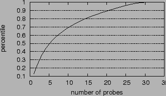
While PlanetSeer's combination of passive monitoring and distributed active probing is very effective at finding anomalies, particularly the short-lived ones, the probing traffic can be aggressive, and can come as a surprise to low-traffic sites that suddenly see a burst of traceroutes coming from around the world. Therefore, we are interested in reducing the measurement overhead while not losing the accuracy and flexibility of our approach. For example, we can use a single traceroute to confirm loops, and then decide if we want distributed traceroutes to test for the presence of correlated loops. Similarly, for path changes and outages, we can reduce the number of distributed traceroutes if we are willing to tolerate some inaccuracy in characterizing their scope. In Figure 10, we plot the CDF of the number of the probes from other vantages points we have to examine before we find the intercept traceroutes that can successfully narrow the scopes of the anomalies. Using only 15 vantage points, we achieve the same results as when using all 30 vantage points in 80% of the cases. We are interested in studying this issue further, so that we can determine which vantage points we need to achieve good results.
There is extensive existing work on studying Internet path failure. Labovitz and Ahuja [15] studied inter-domain routing failures using BGP data collected from several ISPs and 5 network exchange points. They analyzed the temporal properties of failures, such as mean time to fail, mean time to repair and failure duration. They found that 40% of the failures are repaired in 10 minutes and 60% of them are resolved in 30 minutes. They also studied the intra-domain routing failures of a medium-sized regional ISP by examining the data from the trouble ticket tracking system managed by the Network Operation Center (NOC) of the ISP, together with the OSPF routing messages. Based on this data, they characterize the origins of failures into hardware, software and operational problems.
Iannaccone et al. investigated the failures in Sprint's IP backbones using the IS-IS routing updates collected from three vantage points [12]. They examined the frequency and duration of failures inferred from routing updates and concluded that most failures are short-lived (within 10 minutes). They also studied the interval between failures. Again, their focus is on the temporal properties of failure.
Mahajan, Wetherall and Anderson [16] studied BGP misconfigurations using BGP updates from RouteViews [18], which has 23 vantage points across different ISPs. They found BGP misconfigurations were relatively common and classified them into origin and export misconfigurations. Note that BGP misconfigurations may or may not be visible to end users. They observed that only 1 in 25 misconfigurations affect end-to-end connectivity.
More recently, Feldmann et al. have presented a methodology to locate the origin of routing instabilities along three dimensions in BGP: time, prefix, and view [9]. Their basic assumption is that an AS path change is caused by some instability either on the previous best path or the new best path. Caesar et al. [4] and Chang et al. [5] also propose similar approaches to analyze routing changes, although their algorithms are different in details.
All of the above failure studies are based on either inter-domain (BGP) or intra-domain (IS-IS, OSPF) routing messages, from which failures are inferred. Some of them require access to the ISP's internal data, such as trouble tickets. Our study complements this work by studying failures from an end-to-end perspective, and quantifies how failures affect end-to-end performance, such as loss rate and RTT.
There also has been much work on studying Internet failures through end-to-end measurement, and these have greatly influenced our approach. Paxson [19] studied the end-to-end routing behavior by running repeated traceroutes between 37 Internet hosts. His study shows that 49% of the Internet paths are asymmetric and visit at least one different city. 91% of the paths persist more than several hours. He used traceroutes to identify various routing pathologies, such as loops, fluttering, path changes and outages. However these traceroutes do not distinguish between forward and reverse failures.
Chandra et al. [6] studied the effect of network failures on end-to-end services using the traceroute datasets [19,21]. They also used the HTTP traces collected from 11 proxies. They model the failures using their location and duration and evaluate different techniques for masking failures. However, the HTTP and traceroute datasets are independent. In comparison, we combine the passive monitoring data and active probing data, which allows us to detect failures in realtime and correlate the end-to-end effect with different types of failures. They also classify the failures into near-source, near-destination and in-middle by matching /24s IP prefixes with end host IPs. In contrast, we study the location of failures using both IP-to-AS mapping [17] and 5-tier AS hierarchies [23]. This allows us to quantify the failure locations more accurately and at a finer granularity.
Feamster et al. measured the Internet failures among 31 hosts using periodic pings combined with traceroutes [7]. They ping the path between a pair of nodes every 30 seconds, with consecutive ping losses triggering traceroutes. They consider the location of a failure to be the last reachable hop in traceroute and used the number of hops to closest end host to quantify the depth of the failure. They characterize failures as inter-AS and intra-AS and use one-way ping to distinguish between forward and reverse failures. They also examine the correlation between path failures with BGP updates.
Our work is partly motivated by these approaches, but we cannot use
their methodology directly because of environmental differences. With
the large number of clients that connect to our proxies, we can not
afford to ping each of them frequently. Failure detection and
confirmation are more challenging in our case, since many clients may
not respond to pings (behind firewalls) or even are offline (such as
dialup users). We infer anomalies by monitoring the status of active
flows, which allows us to study anomalies on a much more diverse
set of paths. We also combine the baseline traceroutes with passive
monitoring to distinguish between forward and reverse failures and
classify forward anomalies into several categories. Since where the
failure appears may be different from where the failure occurs, we
quantify the scope of failures by correlating the traceroutes from
multiple vantage points, instead of using one hop (last reachable hop)
as the failure location. Finally, we study how different types of
anomalies affect end-to-end performance.
This paper introduces what we believe to be an important new type of diagnostic tool, one that passively monitors network communication watching for anomalies, and then engages widely-distributed probing machinery when suspicious events occur. Although much work can still be done to improve the tool--e.g., reducing the active probes required, possibly by integrating static topology information and BGP updates--the observations we have been able to make in a short time are dramatic.
We have shown that PlanetSeer provides an effective means to detect large numbers of anomalies with broad coverage, especially in the case of wide-area services that cannot rely on cooperation from one endpoint. In addition to the detection rate, the short delay between emergence and detection allows us to capture anomaly behavior more effectively, and our distributed framework provides improved characterization.
This research was supported in part by NSF grant CNS-0335214. We would like to thank KyoungSoo Park for his effort in keeping CoDeeN operational during this work. We thank our shepherd, Miguel Castro, for his guidance and helpful feedback, and we thank our anonymous reviewers for their valuable comments on improving this paper.
|
This paper was originally published in the
Proceedings of the 6th Symposium on Operating Systems Design and Implementation,
December 6–8, 2004, San Francisco, CA Last changed: 18 Nov. 2004 aw |
|