|
USITS '03 Paper
[USITS '03 Tech Program Index]
| Pp. 239-252 of the Proceedings |  |
Network-Sensitive Service Discovery
An-Cheng Huang and Peter Steenkiste
Carnegie Mellon University
{pach,prs}@cs.cmu.edu
Abstract:
We consider the problem of network-sensitive service selection (NSSS): finding
services that match a particular set of functional and network properties.
Current solutions handle this problem using a two-step process.
First, a user obtains a list of candidates through service discovery.
Then, the user applies a network-sensitive server selection technique to
find the best service. Such approaches are complex and expensive
since each user
has to solve the NSSS problem independently.
In this paper, we present a simple alternative: network-sensitive service
discovery (NSSD). By integrating network-sensitivity into the
service discovery process, NSSD allows users who are looking for
services to specify
both the desired functional and network properties at the same time.
Users benefit since they only have to solve a restricted version of
the server selection problem. Moreover,
NSSD can solve
the NSSS problem more efficiently by amortizing the overhead over many users.
We present the design of NSSD, a prototype implementation, and
experimental results that illustrate how NSSD can be utilized for different
applications.
There is considerable interest in network services that are more
sophisticated than traditional Web services. Examples include interactive
services such as video conferencing, distributed games, and distance learning.
An important property of these services is that their performance depends
critically on the network, so the service selection process should consider
the network capabilities, i.e., it should be network-sensitive.
One way of building such sophisticated services is through composition
of service components (e.g., automatic path creation [23]
in Ninja [13], Panda [31], and Libra [34]).
The ``brokers'' that
select and compose the service components also have to consider network
properties, e.g., they should make sure sufficient bandwidth is available
between a component and the users, and between components. The key
operation in these examples is the network-sensitive service selection (NSSS)
problem.
Existing research related to the NSSS problem falls in roughly two
classes. Service discovery infrastructures allow a user
to find a set of servers with
certain functional properties, where the properties are typically
described as a set of attribute-value pairs.
Existing solutions, for example, [16] and [6],
differ in the flexibility of naming
and matching and in their scalability properties.
On the other hand, given a set
of servers that provide a particular service,
the server selection problem is to select the one
that can best satisfy the user's requirements.
Previous work in this area has mostly focused on the problem of
identifying
the Web server that is ``closest'' to a client,
e.g., has the
highest-bandwidth or lowest-latency
path [3,4,21,32].
Clearly we can solve the NSSS problem by combining service discovery and
server selection in the following way.
A user first utilizes a service discovery infrastructure to obtain a list
of servers that can provide the required service
and then applies a server selection technique to identify the
server that can best satisfy the user's requirements.
Unfortunately, this solution is often not practical.
A first problem is scalability:
for common services, the number of servers to be considered in the server
selection phase would be overwhelming, making the process very expensive.
A second problem is complexity: server selection is a difficult problem,
and requiring each user (e.g., application or broker) to develop these
mechanisms from scratch increases the development cost.
Finally, if services are offered by commercial providers, they may not
be willing to expose their individual
servers, so user-side selection cannot be performed.
We propose a simple alternative, namely
network-sensitive service discovery
(NSSD). The idea is that when users contact the service discovery
infrastructure,
they can specify not only static functional properties, but also network
connectivity and server load properties.
NSSD returns the best server (or a small number of good servers) according
to the user's requirements.
Therefore, in effect we have moved most of the
complexity of server selection from the user to the service discovery
infrastructure. Providers do not need to expose all their servers to users,
since server selection is handled by NSSD, which is trusted by the providers.
Moreover, by integrating service discovery and server selection,
NSSD can amortize overhead such as collecting network information
across multiple users and can also apply distributed solutions.
Therefore, we can solve the NSSS problem more efficiently and in a
more scalable way.
The remainder of this paper is organized as follows. We elaborate on
challenges associated with the NSSS problem in the next section.
In Section 3 we describe our network-sensitive service
discovery solution, including the design of the service API and the
mechanisms used for network-sensitive service discovery. We
describe a prototype system in Section 4,
and Section 5 presents an evaluation using the
PlanetLab testbed.
Finally, we discuss related work and summarize.
Let us first identify the players:
- Providers: Each provider provides a service,
for example, a service that provides streaming video of movies.
Typically, a provider will use a set of distributed servers to
deliver the service, for example, a set of replicated streaming servers.
- Users: Each user invokes and uses one or more services.
A user can either be an end user, for example,
a person watching a movie using a streaming video service, or
another service provider, for example, a video streaming service may
rely on another service provider for transcoding service.
For a particular service type, there will typically be many different
providers, each of which may have many servers. In a traditional setup,
a user utilizes a service discovery mechanism to select a
provider that can deliver the required service. The selection of the
specific server can then either
be done by the selected provider (provider-side selection),
or it can be done by the user, assuming the provider makes
information about its internal capabilities available to the user
(user-side selection).
Unfortunately, server selection becomes
more complicated if the selection has to be done in a network-sensitive
fashion or if users want to use user-specific selection criteria.
Before we address these questions,
let us look at some application examples.
2.2 Applications
Figure 1:
Selecting a game server for a multiplayer online game
|
Figure 2:
Proxy-based End System Multicast (ESM) example
|
Figure 3:
Composing a video streaming service
|
In Figure 1, four users
want to play a multiplayer online game together,
so they need a game server to host their gaming session.
Specifically, they need a game server that not only satisfies certain
functional properties (e.g., supports a particular game and has
certain anti-cheating features) but also delivers good
``performance''. For this application, this means that the
players have a low network latency to the server and that the server
is lightly loaded.
In the second example (Figure 2),
a group of users want to use a
proxy-based End System Multicast (ESM, see [5]) service.
Each participant sends its packets to an ESM proxy, and all
proxies serving this group construct an ESM overlay to efficiently
deliver the packets to all other participants. The problem is
finding a set of appropriate ESM proxies to serve the users.
One possible selection metric in this case is the sum of the latencies
between each
user and the ESM proxy assigned to the user, since minimizing this metric may
reduce the total network resource usage.
The third example is a simple service composition scenario
(Figure 3): a user
wants a service that provides low bit rate MPEG-4 video streams, and
we can deliver such a service by putting together a high bit rate
MPEG-2 video streaming service and an MPEG-2-to-MPEG-4 video transcoding
service. If our goal is to minimize the total bandwidth usage,
this scenario presents an interesting situation:
selecting a streaming server close to the user can reduce bandwidth usage,
but a more distant streaming server
may turn out to be a better choice if we can find a transcoder that is
very close to the server. In other words, this problem requires
the coordinated selection of multiple services.
There has been a lot of research on network-sensitive
server selection, i.e., given a list of servers, select the best one
considering certain network properties.
Some approaches perform active probing at selection
time to determine the best server,
for example, [4] and [8], while others
use network properties that have been computed, measured, or observed
earlier,
for example, [3,30,32,33].
Most of these techniques were developed for specific applications,
and they were applied either on the
user side or on the provider side.
In a provider-side approach, a user first utilizes service discovery
to select a provider, and the provider then
internally applies a network-sensitive selection technique to select one of
its servers for the user.
In a user-side approach, a user obtains a list of
candidate servers from the selected provider, and
it then applies network-sensitive selection to select one of the candidates.
Although applying network sensitivity on the user side or the provider side
is suitable for some applications (e.g., user-side Web mirror server
selection, provider-side cache selection in content distribution networks,
etc.), both user-side and provider-side approaches have their
limitations. The advantage of provider-side approaches, i.e., being
transparent to users, is also its disadvantage: a user does not control
the selection criteria and does not know what level of performance can
be expected.
User-side approaches, on the other hand, have high overhead: every user
needs to obtain a potentially long list of candidates and
collect network status information for the candidates. Also,
each application has to implement a network-sensitive selection technique.
Moreover, providers
must release details about their internal capabilities, a dubious
assumption at best.
In this paper, we propose a different approach:
network-sensitive service discovery (NSSD), which integrates
service discovery and network-sensitive server selection.
NSSD allows a user to
specify both functional and network properties when selecting a server.
Given these properties, NSSD returns the best server or a small number of
``good'' candidates to the user.
The user can then use the candidates to perform user-specific optimizations.
There may be competing NSSD
infrastructures, and providers and users can choose which one to use.
A large provider providing many servers/services can even implement its
own NSSD infrastructure.
Compared with provider-side approaches, NSSD allows
users to control the selection criteria, and it exposes sufficient
information to allow users to further optimize the selections (e.g.,
global optimizations in service composition). Compared with user-side
approaches, NSSD has lower overhead both in terms of service discovery
(only a small number of good candidates are returned to the user)
and network sensitivity (NSSD can amortize the cost of
collecting network status information).
In addition, providers only need to release
their complete server information to a ``trusted'' NSSD infrastructure.
3 Network-Sensitive Service Discovery
We define the API used for formulating NSSD queries
and describe several possible NSSD designs.
3.1 NSSD API
To define our API for NSSD, we need to determine what
functionalities NSSD should provide. From the three examples in Section 2.2, we can see that
the server selection problem is
an optimization problem: find a solution
(e.g., a game server) that optimizes a certain metric
(e.g., the maximum latency) for a target or a set of targets
(e.g., the players).
The examples illustrate two types of optimization problems:
local and global.
A local optimization problem involves the selection of a single service,
e.g., select a game server that minimizes the maximum latency to
a group of players. A global optimization problem involves
the coordinated selection of different services,
e.g., select a streaming server and a transcoder such that the overall
bandwidth usage is minimized. Note that in service composition scenarios
(e.g., Figure 3), selecting each service
independently using local
optimizations may not yield the globally optimal solution.
The key question is: what part of the optimization should be done by
NSSD and what part should be left to the user. We decided to
define an API that would allow a user to ask NSSD to perform local
optimizations for individual services using generic optimization metrics.
However, a user can also ask NSSD to return a small number of
``locally good'' candidates for each service so that the user can then
apply global optimization criteria across services using the returned results.
Let us elaborate on these design decisions:
- Local optimization only: Our API allows users to
specify local optimization problems only, i.e., a user can only ask NSSD to
select one
service at a time. The reason for this decision is that
global optimizations are likely to be service-specific and may be
arbitrarily complex, so it is more appropriate
to leave them to the user.
Note, however, that multiple ``identical servers'' may be required to provide
a service.
For example, in Figure 2, we need to select three
ESM proxies for the ESM service, using the sum of the latencies as the
optimization metric.
We consider such optimization problems to be local, and they are supported
by NSSD.
- A set of standard metrics: Our API allows a user
to specify constraints and preferences on a set of standard metrics:
maximum and average latency, minimum and average bandwidth, and server load.
While it may be possible to allow users to specify,
for example, their own utility functions based on these standard metrics,
it is currently not clear that the potential benefit is
worth the extra complexity.
- Best-n-solutions:
As defined by the first two decisions, NSSD supports local optimizations
based on a set of standard metrics. While this is sufficient in many
cases involving the selection of single services, it is not adequate in cases
requiring the coordinated selection of multiple services or the use of
user-specific metrics. Therefore, NSSD also allows a user to ask for
a number of good solutions when selecting a service. The user can then
apply user-specific or global optimization criteria on these locally good
solutions.
In Section 3.2, we will use a service composition
example to illustrate the use of this best-n-solutions feature.
Figure 4:
The NSSD API
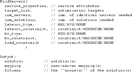 |
Figure 4 shows the resulting NSSD API.
The argument ``num_servers'' specifies how many identical servers
are required in a solution, and ``num_solutions'' specifies how many
locally good solutions should be returned. The solutions are returned
in ``solution'', in the form of IP addresses. When multiple identical
servers are needed in a solution, ``mapping'' specifies which server is
used for each user.
NSSD also returns a ``fitness'' (i.e., the value of the
selection metric) for each returned solution, which may be
helpful to the user for use in further optimizations.
This can be viewed as a compromise between two extremes:
having the provider not release any details about the service it
can provide (which prevents user-specific optimizations) and
having the provider list all its capabilities
(which would be needed for pure user-side optimizations).
Note that a server returned may be the front end of a cluster of servers.
Since servers in a cluster have similar network properties, this
does not affect the effectiveness of the network-sensitive selection in NSSD,
and it leaves room for the provider to do internal load balancing.
Note also that additional information regarding each solution
(e.g., monetary cost) may need to be returned so that the user can
perform further optimizations.
Figure 5:
Using the API in the ESM example
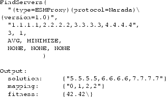 |
Let us use the End System Multicast (ESM) example
in Figure 2 to illustrate the use of the API.
The top part of Figure 5 shows the NSSD query in this
scenario. We first specify that we want to find ESM
proxies that are using the Narada protocol version 1.0. The next parameter
specify that the selection should be optimized for the four users in this
scenario. The next two parameters specify that we want three identical
ESM proxies in a solution,
and we only need the best solution. The remaining
input parameters specify that we want to minimize the average latency,
and we do not have constraints or preferences on bandwidth and load.
Assuming that the best solution is the configuration in
Figure 2,
the result returned by the API is shown in the bottom part of
Figure 5. NSSD returns the best solution, which consists
of three ESM proxies,
and the ``mapping'' specifies that user 1 is assigned to ESM proxy
5.5.5.5, user 2 is assigned to 6.6.6.6, and users 3 and 4 are assigned
to 7.7.7.7. In addition, the fitness value of this solution
is 42.42.
3.2 A Sample Application: Service Composition
Figure 6:
An example of service composition: video conferencing session
|
In this section, we use a more complex example of service composition
to illustrate the use of NSSD.
Suppose the five users in
Figure 6
want to establish a video conferencing session.
The problem
is that they are using different video conferencing applications
and hardware platforms: P1 and P2 are using the MBone applications
vic/SDR,
P3 and P4 are using Microsoft NetMeeting, and P5
is using a handheld device that is receive-only and does not do
protocol negotiation.
We can support this conference by composing a video conferencing service
using the following more
primitive service components.
First, we need a ``video conferencing gateway'' (VGW)
that supports interoperability between H.323, which is used by NetMeeting,
and Session Initiation Protocol (SIP), which is used by SDR.
Second, we need a ``handheld proxy'' (HHP) that can join the session
on behalf of the handheld user and forward the video stream to the
handheld device. Finally, we can use the ESM service
to establish a multicast session among the vic users, the VGW, and
the HHP, as shown in Figure 6.
Note that this is more general than service
composition based on a path model, which is explored in, for example,
the Ninja [23] and Panda [31] projects.
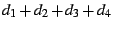
This service composition example raises an interesting challenge:
the selection of the different components is mutually dependent.
For example,
suppose our goal is to minimize the total network resource usage,
and the optimization heuristic we use is to minimize the following function:
where  , ,  , and , and  are weights for the three parts (multicast,
handheld, and NetMeeting) of the service, and
the other variables are the latencies between different nodes
as depicted in Figure 6.
Different weights for the three parts reflect the difference in
bandwidth consumption.
For example, NetMeeting can only receive one video stream, and
the HHP may reduce the video bandwidth before forwarding it to the handheld. are weights for the three parts (multicast,
handheld, and NetMeeting) of the service, and
the other variables are the latencies between different nodes
as depicted in Figure 6.
Different weights for the three parts reflect the difference in
bandwidth consumption.
For example, NetMeeting can only receive one video stream, and
the HHP may reduce the video bandwidth before forwarding it to the handheld.
Unfortunately, selecting all the components together to minimize the above
function may be too expensive to be practical. For example, suppose there
are  VGWs, HHPs, and ESM proxies available. To find the
optimal configuration, we need to look at roughly VGWs, HHPs, and ESM proxies available. To find the
optimal configuration, we need to look at roughly  possible
configurations, which is only feasible when is small.
Therefore, our approach is to use the following heuristic: select
each component using local optimizations and then combine the
locally optimal solutions into a global solution. This is the
approach supported by NSSD. For example, in the video conferencing
service above,
we first ask NSSD to return the VGW that is closest to the NetMeeting
users (since they only support unicast), we then ask NSSD to return the
HHP that is closest to the handheld user, and finally we ask NSSD to
return the optimal set of ESM proxies (minimizing possible
configurations, which is only feasible when is small.
Therefore, our approach is to use the following heuristic: select
each component using local optimizations and then combine the
locally optimal solutions into a global solution. This is the
approach supported by NSSD. For example, in the video conferencing
service above,
we first ask NSSD to return the VGW that is closest to the NetMeeting
users (since they only support unicast), we then ask NSSD to return the
HHP that is closest to the handheld user, and finally we ask NSSD to
return the optimal set of ESM proxies (minimizing
 )
for the vic/SDR users, the selected VGW, and the selected HHP.
In other words, we utilize NSSD to solve three local optimization problems
sequentially (using three local optimization heuristics) and combine the
three local solutions to get a global solution. )
for the vic/SDR users, the selected VGW, and the selected HHP.
In other words, we utilize NSSD to solve three local optimization problems
sequentially (using three local optimization heuristics) and combine the
three local solutions to get a global solution.
Of course, a combination of locally optimal solutions may not be globally
optimal.
To improve the component selection, we can utilize the
``best-n-solutions'' functionality provided by NSSD. For example, in the
video conferencing service, we first ask NSSD to return the best VGWs
(in terms of latency to NetMeeting users), and we then ask NSSD to return
the best (closest to the handheld user)  HHPs. Now we have HHPs. Now we have  possible
VGW/HHP combinations. For each of the combinations, we ask NSSD to
find the optimal set of ESM proxies, and we get a global solution by combining
the VGW, the HHP, and the ESM proxies. Therefore, we have a set of
global solutions, and we can use Function 3.1 to
evaluate them and select the best global solution in this set. possible
VGW/HHP combinations. For each of the combinations, we ask NSSD to
find the optimal set of ESM proxies, and we get a global solution by combining
the VGW, the HHP, and the ESM proxies. Therefore, we have a set of
global solutions, and we can use Function 3.1 to
evaluate them and select the best global solution in this set.
We believe this approach can yield a reasonably good global
solution and allow a provider to
adjust the trade-off between global optimality and optimization cost
by controlling the values of and .
For example, if and are set to 1, the resulting solution is simply
a combination of locally optimal solutions.
On the other hand, if and are the total numbers of VGWs
and HHPs, respectively, we are in fact performing an exhaustive
search in the complete search space, and we will find the
globally optimal solution at a higher cost.
Later in Section 5.4
we will use this video conferencing example to evaluate
the effectiveness of this approach.
3.3 A Simple NSSD Query Processor
Given the NSSD API described in Section 3.1,
NSSD queries can be resolved in many different ways.
In this section, we first describe a
simple approach that heavily leverages earlier work in service
discovery and network measurement; this is also the design
used in our prototype. We mention
alternative approaches in the next section.
Figure 7:
Handling an NSSD query
|
As shown in Figure 7,
a simple NSSD query processor (QP) can be built on top of
a service discovery infrastructure
(e.g., the Service Location Protocol [16]) and
a network measurement infrastructure that can
estimate the network properties (e.g., latency) between nodes.
When the QP module receives an NSSD query (step 1 in
Figure 7), it
forwards the functional part of the query to the service directory
(step 2).
The directory returns a list of candidates that match the functional
properties specified in the query (step 3).
Then the QP module retrieves the necessary network information
(e.g., the latency between each of the candidate and user X)
from the network measurement infrastructure (step 4).
Finally, the QP module computes
the best solution as described below
and returns it to the user (step 5).
One benefit of integrating service discovery and server selection
in a single service is that caching can be used to improve performance
and scalability. When
NSSD gets requests from many users, the cost of collecting
network status information or server load information can be amortized.
Furthermore, network nodes that are close to each other should have
similar network properties. Therefore, nodes can be aggregated to
reduce the amount of information required (for example,
use the same latency for all users in an address prefix).
This should improve the effectiveness of caching.
Selecting the best solution(s) requires solving a fairly general
optimization problem.
Through the NSSD API described earlier, a user can specify
many different combinations of (1) constraints and preferences on three
metrics (latency, bandwidth, and load), (2) how many identical
servers are needed in
a solution, and (3) how many solutions are needed.
The QP computes the solution for a query as follows.
First, the QP applies any constraints in a query to eliminate any
ineligible candidates. Then, the preferences in a query can be
formulated as an optimization problem. If there is only a single
preference, the QP can simply sort the candidates accordingly. If there
are multiple preferences (e.g., minimize load and minimize latency),
there may not be any candidates that satisfy all preferences. One possible
solution is to have the QP define an order among the preferences (e.g.,
in the order they appear in the query) and sort the
candidates accordingly. Finally, if a query requests multiple identical
servers in a solution
(e.g., requesting 3 ESM proxies for 4 users), the optimization problem can
be cast as  -median, -center,
or set covering problems [7], which are more expensive to solve. -median, -center,
or set covering problems [7], which are more expensive to solve.
The above NSSD design is only one option.
Here we briefly describe three distributed implementations.
A content discovery system based on hashing is described
in [12]. The system uses a hash-based overlay network mechanism
(such as Chord [35]) to allow publishers and subscribers
to find each other in rendezvous points based on common attribute-value
pairs, which may be dynamic.
Therefore, it can also be used as a
service discovery infrastructure, and one can incorporate network sensitivity
into the query resolution phase of the system so that the returned matches
satisfy certain network properties specified in the query.
Another alternative is application-layer anycasting [38],
in which each service is represented by an anycast domain name (ADN).
A user submits an ADN along with a server selection filter (which specifies
the selection criteria) to an anycast resolver, which resolves the ADN to
a list of IP addresses and selects one or more from the list using
the filter. Potentially, the ADN and resolvers can be extended to
allow users to specify the desired service attributes, and the filter
can be generalized to support more general metrics.
Finally, distributed routing algorithms are highly scalable, and they
can, for example, be used to find a path that satisfies
certain network properties and also includes a server with certain
available computational resources [19].
A generalization of this approach can be combined with a service discovery
mechanism to handle NSSD queries.
4 Implementation
We describe a prototype NSSD based on
Service Location Protocol (SLP) [16] and
Global Network Positioning (GNP) [24].
We have experimented with versions of our NSSD implementation
on the ABone [1], Emulab [9],
and PlanetLab [29] testbeds.
4.1 Extending SLP
Our implementation of NSSD is based on OpenSLP [26], an
implementation of SLP.
Available services register
their information (location, type, and attributes) with a Directory Agent
(DA), and users looking for services send queries (specifying the
type and attributes of the desired services) to the DA.
Service types and attributes are well known so that a user knows what
to ask for. SLP query specification is quite general:
attributes can be specified as
an LDAPv3 search filter [18], which supports, for example, logical
operations, inequality, and substring match. Therefore, a user query
includes a service type (e.g., ``GameServer'') and a filter,
e.g., ``(&(game=Half-Life)(mod=Counter-Strike)(version =1.5))''.
We believe this query representation is sufficiently general to support
NSSD queries as defined by the API in Section 3.1. =1.5))''.
We believe this query representation is sufficiently general to support
NSSD queries as defined by the API in Section 3.1.
Figure 8:
A sample filter for the game example
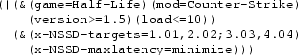 |
In order to support NSSD queries, we extended the semantics of the SLP filter
to include a set of special attributes, representing the
parameters described in Figure 4.
For example, suppose a user wants to find a game server that (1) matches
certain service attributes, (2) is serving
at most ten sessions, and (3) minimizes the maximum latency for
the two players whose GNP coordinates are ``1.01,2.02'' and
``3.03,4.04'', respectively. These parameters can be specified
by the filter shown in Figure 8.
The original SLP API returns a list of ``service URLs'' [15].
To return additional information about
each selected server, we simply add the information to the end of the URLs.
For example, to return the mapping, the DA can return the following
service URL: ``service:GameServer://192.168.0.1;x-NSSD-mapping=0,0,0,0''.
Since server load is also a service attribute, each server's
registration includes the load attribute (e.g., ``load=0.5'').
When conducting ``live'' experiments (i.e., involving applications running
on actual network hosts),
we need mechanisms to dynamically update the load value of
each server. Our live experiments are developed and conducted on the
PlanetLab wide-area testbed [29],
which allows us shell access on about 70 hosts at nearly 30 sites.
We implemented a ``push-based'' load update mechanism:
servers push their load information
(in the form of a registration update) to the DA.
In our evaluation, we look at how the frequency of load update affects
the performance of the server selection techniques.
4.2 Network Measurement
A network measurement infrastructure provides a way for users to obtain
network information.
A number of such infrastructures have been proposed, for example,
IDMaps [11] and Global Network Positioning (GNP) [24].
Most of these infrastructures
only provide latency information. Since it is in general much
harder to estimate the bandwidth between two network nodes,
we currently focus on dealing with the latency metric.
In our implementation, we use GNP as the network measurement infrastructure
to provide latency (round trip time) information between two network
nodes. The key idea behind GNP is to model the Internet as a geometric
space using a set of ``landmark nodes'',
and each network host can compute its own coordinates by probing the
landmarks. It is then straightforward
to compute the distance (latency) between two hosts given their coordinates.
Since the PlanetLab testbed is our current platform, we use the GNP approach
to obtain a set of coordinates for every PlanetLab node.
In the GNP model, each node computes its own coordinates. Therefore,
in our implementation, we use GNP coordinates as a service attribute,
i.e., when a server register with the SLP DA, the registration
includes the coordinates of the server node. When a user specifies the
list of optimization targets in a query (see the API in
Section 3.1), each target is specified in the form of GNP
coordinates.
When a QP asks for a list of candidates, the DA returns the list along
with the coordinates of each candidate.
The advantage of this design is that since the coordinates are computed
off-line, and the latency information can be derived from the coordinates
directly, the cost of querying the network measurement infrastructure at
runtime is eliminated.
A QP can simply use the candidates' and the targets' coordinates
to solve the particular optimization problem specified by a user.
4.3 Selection Techniques
The API defined in Section 3.1 can be used to specify a wide
range of selection techniques.
Below we list the selection techniques that are currently implemented in
our QP and used in our evaluation
( denotes the number of identical servers needed in a solution,
and denotes the number of locally good solutions needed). denotes the number of identical servers needed in a solution,
and denotes the number of locally good solutions needed).
- ``
 , ,  , minimize load'' (MLR):
find the server with the lowest load. If there are multiple servers with
the same load, select one randomly. , minimize load'' (MLR):
find the server with the lowest load. If there are multiple servers with
the same load, select one randomly.
- ``, , minimize maximum latency'' (MM):
find the server that minimizes the maximum latency to the specified target(s).
- ``, , load constraint
 , minimize maximum latency''
(LCxMM):
among the servers that satisfy the specified load constraint
(load , minimize maximum latency''
(LCxMM):
among the servers that satisfy the specified load constraint
(load  ), find the
one that minimizes the maximum latency to the specified target(s). ), find the
one that minimizes the maximum latency to the specified target(s).
- ``, , minimize load, minimize maximum latency''
(MLMM):
find the server with the lowest load, and use maximum latency as the
tiebreaker.
- ``
 , , minimize average latency''
(PMA): find a set of servers
and assign each target to a server so that the average latency between each
target and its assigned server is minimized
(i.e., the -median problem [7]). , , minimize average latency''
(PMA): find a set of servers
and assign each target to a server so that the average latency between each
target and its assigned server is minimized
(i.e., the -median problem [7]).
- ``,
 , minimize average latency''
(MMA): find the best servers
in terms of the average latency between server and each user. , minimize average latency''
(MMA): find the best servers
in terms of the average latency between server and each user.
- ``Random'' (R): randomly select a server.
In the evaluation section, we use these techniques to solve the NSSS
problem for different applications.
5 Evaluation
We present the results of experiments that quantify
how well our NSSD prototype can support two sample applications.
First, we use a multiplayer gaming application to illustrate the
importance of network-sensitive server selection and to show the relative
performance of the different selection mechanisms in our prototype.
Next we use the service composition example of
Section 3.2 to show the trade-offs between local
and global optimizations.
We also present the computational overhead of the NSSD prototype.
The gaming service experiments are conducted on the
PlanetLab wide-area testbed [29].
The service composition experiments are simulations based on latency
measurement data from the Active Measurement Project at
NLANR [25].
In the first set of experiments, we look at how network sensitivity can help
improve application performance. We implemented a simple ``simulated''
multiplayer game client/server: a number of game clients join a session
hosted by a game server, and every 100ms each client sends a small UDP
packet to the hosting server, which processes the packet,
forwards it to all other participants in the session, and
sends an ``ACK'' packet back to the sender.
Our performance metric for the gaming service is
the maximum latency from the server to all clients
since we do not want sessions in which some players are very close
to the server while others experience high latency.
Note that the latency metric is measured from the time that
a packet is sent by a client to the time that the ACK from the server is
received by the client.
The goal of this set of experiments is to evaluate the role of network
performance in the server selection process.
Therefore, we minimized the computation
overhead in the game server to ensure that the server computation power,
including the number of servers, does not affect game performance.
We compare four different scenarios. First, we consider two scenarios,
each of which has 10 distributed servers selected from PlanetLab nodes.
The MM and R
techniques are applied in the two scenarios, respectively.
For comparison, we also consider two centralized cluster scenarios,
CAM and CMU,
each of which has a 3-server cluster, and a random server is selected
for each session.
In the CAM scenario, the cluster is located at the University of Cambridge;
in the CMU scenario, the cluster is at CMU.
The user machines are randomly selected from 50 PlanetLab nodes.
Figure 9:
Central cluster vs. distributed servers in a multiplayer game application
|
Figure 9 shows the average maximum latency
(of 100 sessions) as a function of the number of participants in each session.
MM consistently has the lowest maximum latency, confirming that
network-sensitive
service discovery can successfully come up with the best solution.
More specifically, the results illustrate that
being able to choose from a set of distributed servers
(MM outperforms CMU and CAM)
in a network-sensitive fashion (MM outperforms R) is a win.
Interestingly,
having distributed servers is not necessarily better than a centralized
solution.
In our case, a centrally-located cluster (CMU) outperforms a distributed
network-``insensitive'' solution (R).
Figure 10:
Effect of per-packet processing: average maximum latency
|
Figure 11:
Effect of per-packet processing: average rank
|
Figure 12:
Cumulative distribution under 15 units per-packet processing
|
While the focus of this paper is not on new selection techniques, we
next show how NSSD can easily support different techniques.
We use the simulated game applications
to compare the effectiveness of different selection techniques in NSSD.
We look at the techniques
MLR, MM, LC3MM, MLMM, and R described in
Section 4.3. (LC3MM has load constraint 3, which
means that only servers serving no more than three sessions are eligible.)
Ten nodes at 10 different sites are used as
game servers, 50 other nodes are game clients, and there are four
randomly selected participants in each session. There are on average 10
simultaneous sessions at any time, and the server load information
in the DA's database is updated immediately, i.e., each server's load
value is updated whenever it changes (we relax this in the next section).
We ran measurements for different per-packet processing overhead, which we
controlled by changing the number of iterations of a computationally
expensive loop. The unit of the processing overhead corresponds roughly
to 1% of the CPU (when hosting a 4-participant session).
For example, on a server that is hosting a single 4-participant session
with 10 units of per-packet processing overhead, the CPU load
is about 10%.
Figure 10 shows the
average maximum latency (of 200 sessions) as a function of the
per-packet processing cost. R and MLR have almost identical
performance, which
is expected since in this case MLR evenly distributes sessions based on
the number of gaming sessions on each server.
MM and LC3MM are also almost identical when the per-packet processing
is low. However, the performance of MM degrades
rapidly at higher loads, while LC3MM remains the best performer throughout
this set of experiments.
Figure 11 shows the results from a different perspective:
it shows the average ``rank''
of the five techniques, i.e., for each session, we rank
the techniques from 1 to 5 (best to worst), and we then average over
the 200 sessions. We see that although
the rank of MM gets worse for higher loads, it is still better
than R and MLR at the highest load, despite the fact that its average is
much worse than those of R and MLR. The reason can be seen in
Figure 12, which compares the cumulative distributions
of the maximum latency of R, MM, and LC3MM for the case of 15 units
per-packet
processing. It shows that MM in fact makes many good selections, which
helps its average rank. However, the 10% really bad choices
(selecting overloaded
servers) hurt the average significantly. In contrast, LC3MM consistently
makes good selections, which makes it the best performer both in terms of
average and rank.
Figure 13:
Effect of load update frequency: average maximum latency
|
Figure 14:
Effect of load update frequency: average rank
|
In the previous set of experiments, the server load information stored in
the DA's database is always up-to-date, which is not feasible in
practice. We now look at how the load update
frequency affects the performance of the selection techniques.
The experimental set up is the same as that in the previous section,
except that we fix the per-packet processing to 15 units and
vary the load update interval,
which is defined as the number of system-wide ``load changes''
between two consecutive
updates of the load information on the DA.
Note that load changes include both establishing a new session and
terminating an old session.
We experimented with three different update intervals: 1 (i.e.,
immediate updates, as in the previous set of experiments),
4, and 8. Since there are on average
10 simultaneous sessions at any time, an update interval
of 8 means that when an update occurs,
40% of the active sessions have been replaced since the previous update.
Figure 13 shows the average maximum latency
for the different techniques using different update intervals.
Since R and MM are not affected by load, we show the data from the previous
set of experiments for comparison. We see that as the update interval
becomes longer, the performance of both LC3MM and MLMM degrades significantly
since they make decisions based on stale load information.
They are worse than R under longer update intervals.
However, in Figure 14, LC3MM and
MLMM consistently have a better average rank than R. The reason is
that when the load update interval is long, LC3MM and MLMM
occasionally make really bad choices, which greatly affect the average
numbers.
5.4 Local Optimization vs. Global Optimization
In the last set of experiments, we use NSSD in the
service composition scenario
described in Section 3.2.
As depicted in Figure 6, we need to find
a video conferencing gateway (VGW), a handheld proxy (HHP), and a set
of ESM proxies. We use the heuristic described in
Section 3.2:
first, we ask NSSD to select the best VGWs using the
MMA technique (see Section 4.3), and
then we ask NSSD to select the best HHPs using MMA.
For each of the VGW/HHP combinations,
we ask NSSD to find the optimal set of ESM proxies using the PMA technique.
Finally, we evaluate the resulting global solutions using
Function 3.1 and select the best one.
Since we are only interested in the global optimality (as defined by
Function 3.1) of the resulting service instances,
we do not need to
run the various components on actual machines. Therefore,
our experiments are based on simulations using the
latency measurement data from the NLANR Active Measurement
Project [25]. The data consists of round trip time measurements
from each of 130 monitors (mostly located in the U.S.)
to all the other monitors.
We process the data to generate a latency
matrix for 103 sites, and then in the simulations we randomly select nodes
from these sites to represent users and various components.
Next, we present the results from three sets of experiments
and compare them.
In the weighted-5 set, we use weights 5.0, 2.0, and 1.0 for , ,
and , respectively.
We select
40 random nodes as client nodes, 5 random nodes as VGWs, 5 as HHPs, and
5 as ESM proxies (these 4 sets are disjoint). We then generate 100
sessions by selecting 5 participants (2 vic/SDR, 1 handheld, and 2 NetMeeting)
from the client nodes for each session. For each session,
we vary the values of and
(from 1 to 5) and compute the corresponding global solutions.
This process (node selection/session generation/simulation) is repeated
20 times, resulting in 20 simulation configurations.
The performance metric is ``relative global optimality'', which is defined
as the value of Function 3.1 for a solution divided by
the value for the globally optimal solution. For example,
a solution with
relative global optimality 1.25 is 25% worse than the globally optimal
solution.
Let us first look at all 100 sessions in a typical simulation
configuration. We experimented with four different settings for  :
(1,1), (2,2), (3,3), and (4,4), and
the results from a typical configuration are :
(1,1), (2,2), (3,3), and (4,4), and
the results from a typical configuration are
Figure 15:
Relative global optimality for sessions in a typical weighted-5 configuration
|
plotted in Figure 15.
For each setting,
the sessions are sorted according to
their relative global optimality (rank 1 to 100, i.e., best to worst).
When is (1,1), we are able to find the globally optimal solution
for 27 sessions, and the worst-case relative global optimality is 1.19.
We can see that as we increase the size of the search space using the
best-n-solutions feature of NSSD, we not only increase the chance of
finding the globally optimal solution but also improve the worst-case
performance.
Therefore, the result demonstrates the effectiveness of our
approximate approach.
Next, we want to look at the results for all sessions in all 20
simulation configurations using all settings.
Figure 16:
Relative global optimality for weighted-5
|
The average relative global optimality result is shown in
Figure 16.
Each data point is the average of 20 configurations,
each of which is the average of 100 sessions.
We decided to present the average (mean)
relative global optimality for each setting instead of the median
value because (as we can see in Figure 15)
the median value often can not show the difference in the performance of
different settings.
When is (1,1),
the resulting solution
is on average 13.7% worse than the globally
optimal solution. When we use (2,2) for , we are performing
an exhaustive search in 16% of the complete search space, and the
resulting solution is 5.3% worse than the globally optimal solution.
The weighted-25 setup is the same as weighted-5 above except that
we use 25 VGWs, 25 HHPs, and 25 ESM proxies for this set.
Figure 17:
Relative global optimality for weighted-25
|
Figure 17 shows
the average relative global optimality for this set of experiments.
When we set to (1,1) and (10,10), the average
relative global optimality of the resulting solution
is 1.279 and 1.035, respectively (i.e., 27.9% and 3.5% worse than the
globally optimal solution).
The unweighted-25 set is the same as weighted-25 above except that
the weights , , and in the global optimization function
(Function 3.1) are all set to 1.0.
Figure 18:
Relative global optimality for unweighted-25
|
The average relative global optimality result is shown in
Figure 18.
When we set to (1,1) and (10,10), the resulting solution is on average
5.9% and 0.1% worse than the globally optimal solution, respectively.
A comparison between weighted-5 and weighted-25 illustrates a few points.
First, although using the combination of locally optimal solutions can
greatly reduce the cost of solving the selection problem, it can lead to
bad solutions (in terms of global optimality).
Second, using the best-n-solutions feature of NSSD
is effective, as we can significantly improve the global optimality of
the resulting solution by searching in a relatively small space.
Third, the performance at (1,1)
seems to degrade as the complete search space becomes larger
(1.137 in weighted-5 and
1.279 in weighted-25). On the other hand,
the effectiveness of the best-n-solutions approach
seems to increase with the size of the complete search space,
e.g., when searching only 16% of the
complete search space (i.e., when we set to (2,2) and (10,10) in
weighted-5 and weighted-25, respectively),
the improvement in weighted-25 is greater than
in weighted-5 (27.9%
 3.5% vs. 13.7%
5.3%). 3.5% vs. 13.7%
5.3%).
When comparing weighted-25 with unweighted-25, we see that in unweighted-25,
the performance at (1,1) is much better than that in weighted-25
(1.059 vs. 1.279),
and increasing and improves the global optimality much faster
than it does in weighted-25, e.g., 5.9%
1.0% vs.
27.9%
12.6% when is (4,4).
An intuitive explanation of this significant difference between the weighted
and the unweighted configurations is that, in this video conferencing
service composition example, the unweighted global optimization function
is actually quite close to the sum of the local optimization metrics
used to select the individual services. As a result, a ``locally good''
candidate is very likely to also be ``globally good''. On the other hand,
in the weighted configuration, the global optimality of a solution
is less dependent on the local optimality of each component, and therefore,
we need to expand the search space more to find good global solutions.
To verify this explanation,
we look at how likely each particular VGW/HHP combination
results in the globally optimal solution. Specifically, for each
of the 2000 sessions, we look at which VGW/HHP combination
(according to their local ranks, e.g., the combination of
the
i-th ranked VGW and the
j-th ranked HHP)
results in the globally optimal solution. Then we aggregate the results
and present, for all
 and and
 ,
the fraction of time that the combination of
the
i-th ranked VGW and the
j-th ranked HHP results in the
globally optimal solution. ,
the fraction of time that the combination of
the
i-th ranked VGW and the
j-th ranked HHP results in the
globally optimal solution.
Figure 19:
Fraction of time each VGW/HHP combination is globally optimal (unweighted-25)
|
Figure 19 shows that in unweighted-25,
nearly 30% of the time simply using the best VGW (rank 1) and
the best HHP (rank 1) results in the globally optimal solution.
Similarly, about 11% of the time using the 2nd-ranked VGW
and the 1st-ranked HHP
results in the globally optimal solution, and so on.
In fact, in unweighted-25,
the vast majority of globally optimal solutions involve
the best few VGWs and HHPs.
On the other hand,
Figure 20:
Fraction of time each VGW/HHP combination is globally optimal (weighted-25)
|
Figure 20 shows the results for weighted-25.
Although using the combination of
the 1st-ranked VGW and the 1st-ranked HHP is still more likely to
result in the globally optimal solution than any other VGW/HHP combinations,
the fraction is now only 4.3%.
Furthermore, the distribution is much more dispersed.
Therefore, these results match our intuition.
We used the ESM scenario of Figure 2 to evaluate the
overhead of the NSSD implementation.
We register 12 ESM proxies (and 24 other services) with NSSD.
Each query asks NSSD to select three ESM proxies for four
random participants while minimizing the average latency between
each participant and its assigned ESM proxy. The queries are generated
using a Perl script and
sent (through a FIFO) to another process that uses the SLP API to send the
queries to the service directory. The replies flow in
the reverse direction back to the Perl script.
All the processes are running on a single desktop machine
(CPU: Pentium III 933MHz).
We measure the total time of generating and processing 4000 back-to-back
queries, and the average (over 10 runs) is 5.57 seconds
(with standard deviation 0.032),
which shows that in this set up NSSD can process roughly
718 queries per second. We believe this is a reasonable number given
the complexity of selecting the ESM proxies and the fact that the time
also includes the overhead of query generation and IPC.
6 Related Work
We summarize related work in the areas of service
discovery, network measurement infrastructure, and server selection techniques.
There have been many proposals for service discovery infrastructures.
For example, Service Location Protocol [16], Service Discovery
Service [6], and Java-based Jini [20]. A distributed
hashing-based content discovery system such as [12] can also
provide service discovery functionality. These
general service discovery infrastructures only support service lookup
based on functional properties, not network properties.
Naming-based approaches for routing client requests to appropriate servers
can also provide service discovery functionality.
Application-layer anycasting [38] performs server
selection during anycast domain name resolution.
In TRIAD [14], requests are routed
according to the desired content and routing metrics.
The Intentional Naming System [2]
resolves intentional names, which are based on
attribute-value pairs, and routes requests accordingly.
Active Names [36] allows clients and service providers
to customize how resolvers perform name resolution.
NSSD can potentially be built on top of the
service discovery and server selection mechanisms in these approaches.
An important part of NSSD is the
network measurement infrastructure, which provides
estimates of network properties such as latency between hosts.
A number of research efforts focus on such an
infrastructure.
For example, in IDMaps [11], the distance between two hosts
is estimated as the distance from the hosts to their nearest ``tracers''
plus the distance between the tracers.
GNP [24] utilizes a coordinates-based approach.
Remos [22] defines and implements an API for providing network
information to network-aware applications.
Many network-sensitive server selection techniques have been studied before.
For example,
in [4]
a number of probing techniques are proposed
for dynamic server selection.
Client clustering using BGP routing information [21] or
passive monitoring [3] has been applied to server selection.
Similarly, distributed binning [30] can be used to identify
nodes with similar network properties.
In SPAND [32], server selection is based on passive monitoring
of application traffic.
The effectiveness of DNS-based server selection
is studied in [33].
Network-layer anycast [28] handles network-sensitive selection at
the routing layer.
The Smart Client architecture [37] utilizes a service-specific
applet to perform server selection for a user (primarily for load-balancing
and fault-transparency).
The performance of various selection techniques is evaluated
in [17] and [8].
These studies provide new ways of collecting and using network information
for server selection and are complementary to our work.
Some other efforts address the problem of request distribution in a server
cluster, for example, [10] and [27]. They are also
complimentary to NSSD since all nodes
within the same cluster have similar network properties.
7 Conclusion
For many applications, the ability to find a server (or a set of servers)
that satisfies a set of functional and network properties
is very valuable.
In this paper, we have proposed an integrated solution: network-sensitive
service discovery (NSSD).
NSSD allows users to benefit from network-sensitive selection
without having to implement their own selection techniques, and it does not
require providers to expose all their server information to users.
The local optimization techniques supported by NSSD can be used in common
cases involving the selection of individual servers, and the best-n-solutions
feature provides additional information that allows users to perform
user-specific global optimizations.
In our evaluation, we show that our prototype implementation of
NSSD has reasonably good query processing performance.
Experimental results for game server selection show that by using
the local optimization functionality provided by
NSSD, the simulated multiplayer
game can get significant performance improvements.
Simulation results for service composition
demonstrate that NSSD also provides the
flexibility for users to approximate the performance of global optimizations
using results from local optimizations.
By using the best-n-solutions feature, a user can perform global optimizations
in a small search space and greatly improve the performance of the
resulting solution.
Acknowledgments
This work was supported in part by the Defense Advanced Research Project
Agency and monitored by AFRL/IFGA, Rome NY 13441-4505, under contract
F30602-99-1-0518. Additional support was provided by Intel.
We thank the organizations hosting the PlanetLab testbed for their support.
We also thank the National Laboratory for Applied Network Research for
providing the latency measurement data, which was sponsored by
National Science Foundation Cooperative Agreement No. ANI-9807479.
We would like to thank Tze Sing Eugene Ng for his help on GNP related issues,
his implementation of a heuristic search algorithm, and his comments on
earlier drafts of this paper.
- 1
-
Active Network Backbone (ABone).
https://www.isi.edu/abone/.
- 2
-
W. Adjie-Winoto, E. Schwartz, H. Balakrishnan, and J. Lilley.
The design and implementation of an intentional naming system.
In Proceedings of ACM SOSP '99, Dec. 1999.
- 3
-
M. Andrews, B. Shepherd, A. Srinivasan, P. Winkler, and F. Zane.
Clustering and Server Selection using Passive Monitoring.
In Proc. IEEE INFOCOM 2002, June 2002.
- 4
-
R. Carter and M. Crovella.
Server Selection Using Dynamic Path Characterization in Wide-Area
Networks.
In Proceedings of IEEE INFOCOM '97, Apr. 1997.
- 5
-
Y. Chu, S. Rao, and H. Zhang.
A Case for End System Multicast.
In Proceedings of ACM Sigmetrics, June 2000.
- 6
-
S. E. Czerwinski, B. Y. Zhao, T. Hodes, A. D. Joseph, and R. Katz.
An Architecture for a Secure Service Discovery Service.
MobiCOM '99, Aug. 1999.
- 7
-
M. S. Daskin.
Network and Discrete Location: Models, Algorithms, and
Applications.
John Wiley & Sons, Inc., 1995.
- 8
-
S. G. Dykes, C. L. Jeffery, and K. A. Robbins.
An Empirical Evaluation of Client-side Server Selection Algorithms.
In Proc. of IEEE INFOCOM 2000, Mar. 2000.
- 9
-
The Emulab testbed.
https://www.emulab.net.
- 10
-
A. Fox, S. Gribble, Y. Chawathe, and E. A. Brewer.
Cluster-Based Scalable Network Services.
In Proceedings of ACM SOSP '97, Oct. 1997.
- 11
-
P. Francis, S. Jamin, C. Jin, Y. Jin, D. Raz, Y. Shavitt, and L. Zhang.
IDMaps: A Global Internet Host Distance Estimation Service.
IEEE/ACM Trans. on Networking, 9(5):525-540, 2001.
- 12
-
J. Gao and P. Steenkiste.
Rendezvous Points-Based Scalable Content Discovery with Load
Balancing.
In Proceedings of NGC 2002, Oct. 2002.
- 13
-
S. D. Gribble, M. Welsh, R. von Behren, E. A. Brewer, D. Culler, N. Borisov,
S. Czerwinski, R. Gummadi, J. Hill, A. Joseph, R. Katz, Z. Mao, S. Ross, and
B. Zhao.
The Ninja Architecture for Robust Internet-Scale Systems and
Services.
IEEE Computer Networks, Special Issue on Pervasive Computing,
35(4), Mar. 2001.
- 14
-
M. Gritter and D. R. Cheriton.
An Architecture for Content Routing Support in the Internet.
In Proceedings of USITS 2001, Mar. 2001.
- 15
-
E. Guttman, C. Perkins, and J. Kempf.
Service Templates and Service: Schemes.
RFC 2609, June 1999.
- 16
-
E. Guttman, C. Perkins, J. Veizades, and M. Day.
Service Location Protocol, Version 2.
RFC 2608, June 1999.
- 17
-
J. Guyton and M. Schwartz.
Locating Nearby Copies of Replicated Internet Servers.
In Proceedings of ACM SIGCOMM '95, Aug. 1995.
- 18
-
T. Howes.
The String Representation of LDAP Search Filters.
RFC 2254, Dec. 1997.
- 19
-
A.-C. Huang and P. Steenkiste.
Distributed Load-Sensitive Routing for Computationally-Constrained
Flows.
In Proceedings of ICC 2003 (to appear), May 2003.
- 20
-
Jini[tm] Network Technology.
https://wwws.sun.com/software/jini/.
- 21
-
B. Krishnamurthy and J. Wang.
On Network-Aware Clustering of Web Clients.
In Proceedings of ACM SIGCOMM 2000, Aug. 2000.
- 22
-
B. Lowekamp, N. Miller, D. Sutherland, T. Gross, P. Steenkiste, and J. Subhlok.
A Resource Query Interface for Network-Aware Applications.
7th IEEE Symposium on High-Performance Distributed Computing,
July 1998.
- 23
-
Z. M. Mao and R. H. Katz.
Achieving Service Portability in ICEBERG.
IEEE GlobeCom 2000, Workshop on Service Portability
(SerP-2000), 2000.
- 24
-
T. S. E. Ng and H. Zhang.
Predicting Internet Network Distance with Coordinates-Based
Approaches.
In Proceedings of IEEE INFOCOM 2002, June 2002.
- 25
-
Active Measurement Project (AMP), National Laboratory for Applied Network
Research.
https://watt.nlanr.net/.
- 26
-
OpenSLP Home Page.
https://www.openslp.org/.
- 27
-
V. Pai, M. Aron, G. Banga, M. Svendsen, P. Druschel, W. Zwaenepoel, and
E. Nahum.
Locality-aware Request Distribution in Cluster-based Network
Servers.
In Proceedings of ASPLOS-VIII, Oct. 1998.
- 28
-
C. Partridge, T. Mendez, and W. Milliken.
Host Anycasting Service.
RFC 1546, Nov. 1993.
- 29
-
PlanetLab Home Page.
https://www.planet-lab.org/.
- 30
-
S. Ratnasamy, M. Handley, R. Karp, and S. Shenker.
Topologically-Aware Overlay Construction and Server Selection.
In Proceedings of IEEE INFOCOM 2002, June 2002.
- 31
-
P. Reiher, R. Guy, M. Yarvis, and A. Rudenko.
Automated Planning for Open Architectures.
In Proceedings for OPENARCH 2000 - Short Paper Session, pages
17-20, Mar. 2000.
- 32
-
S. Seshan, M. Stemm, and R. H. Katz.
SPAND: Shared Passive Network Performance Discovery.
In Proceedings of USITS '97, Dec. 1997.
- 33
-
A. Shaikh, R. Tewari, and M. Agrawal.
On the Effectiveness of DNS-based Server Selection.
In Proc. of IEEE INFOCOM 2001, Apr. 2001.
- 34
-
P. Steenkiste, P. Chandra, J. Gao, and U. Shah.
An Active Networking Approach to Service Customization.
In Proceedings of DARPA Active Networks Conference and
Exposition (DANCE'02), pages 305-318, May 2002.
- 35
-
I. Stoica, R. Morris, D. Karger, M. F. Kaashoek, and H. Balakrishnan.
Chord: A Scalable Peer-to-peer Lookup Service for Internet
Applications.
In Proceedings of ACM SIGCOMM 2001, Aug. 2001.
- 36
-
A. Vahdat, M. Dahlin, T. Anderson, and A. Aggarwal.
Active Names: Flexible Location and Transport of Wide-Area
Resources.
In Proceedings of USITS '99, Oct. 1999.
- 37
-
C. Yoshikawa, B. Chun, P. Eastham, A. Vahdat, T. Anderson, and D. Culler.
Using Smart Clients to Build Scalable Services.
In Proceedings of USENIX 1997 Annual Technical Conference, Jan.
1997.
- 38
-
E. W. Zegura, M. H. Ammar, Z. Fei, and S. Bhattacharjee.
Application-Layer Anycasting: A Server Selection Architecture and
Use in a Replicated Web Service.
IEEE/ACM Trans. on Networking, 8(4):455-466, Aug. 2000.
An-Cheng Huang
2003-01-17
|

![\includegraphics[width=1.6in, keepaspectratio]{gameexample.eps}](img1.png)
![\includegraphics[width=2.0in, keepaspectratio]{esmexample.eps}](img2.png)
![\includegraphics[width=2.8in, keepaspectratio]{mpegcomposition.eps}](img3.png)
![\includegraphics[width=3.0in, keepaspectratio]{composition_example.eps}](img6.png)


![\includegraphics[width=3.0in, keepaspectratio]{nssddirectory.eps}](img19.png)
![\includegraphics[width=3.0in, keepaspectratio]{exp-set1.eps}](img30.png)
![\includegraphics[width=3.0in, keepaspectratio]{exp-set2.eps}](img31.png)
![\includegraphics[width=3.0in, keepaspectratio]{exp-set2-r.eps}](img32.png)
![\includegraphics[width=3.0in, keepaspectratio]{exp-set2-dist.eps}](img33.png)
![\includegraphics[width=3.0in, keepaspectratio]{exp-set3.eps}](img34.png)
![\includegraphics[width=3.0in, keepaspectratio]{exp-set3-r.eps}](img35.png)
![\includegraphics[width=3in, keepaspectratio]{exp-LvG-w5-dist.eps}](img37.png)
![\includegraphics[trim= 112 0 0 0, width=3.65in, keepaspectratio, clip]{exp-LvG-diff-w5.eps}](img38.png)
![\includegraphics[trim= 95 0 0 0, width=3.65in, keepaspectratio, clip]{exp-LvG-diff-w25.eps}](img39.png)
![\includegraphics[trim= 95 0 0 0, width=3.65in, keepaspectratio, clip]{exp-LvG-diff-nw25.eps}](img40.png)
![\includegraphics[trim= 50 0 0 0, width=3.6in, keepaspectratio, clip]{exp-LvG-prob-nw25.eps}](img46.png)
![\includegraphics[trim= 50 0 0 0, width=3.6in, keepaspectratio, clip]{exp-LvG-prob-w25.eps}](img47.png)