
 |
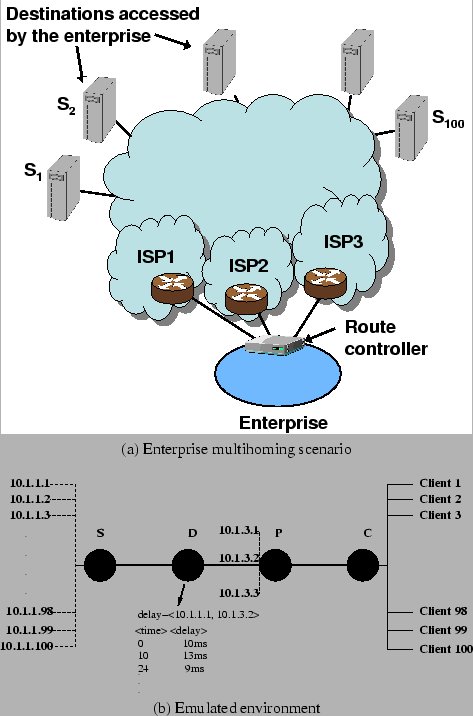 |
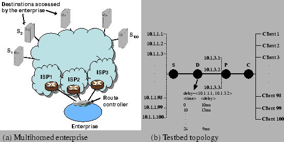
We use the simple testbed topology shown in Figure 4(b). Our goal is to emulate a moderately-sized enterprise with three provider connections and a client population of about 100 (shown in Figure 4(a)).
Node ![]() in the topology runs a simple lightweight Web server and has
one network interface configured with 100 different IP aliases -
10.1.1.1 through 10.1.1.100. Each alias represents an instance of a
Web server - 10.1.1.1 being the most popular and 10.1.1.100 being the
least popular.
in the topology runs a simple lightweight Web server and has
one network interface configured with 100 different IP aliases -
10.1.1.1 through 10.1.1.100. Each alias represents an instance of a
Web server - 10.1.1.1 being the most popular and 10.1.1.100 being the
least popular.
Node ![]() runs 100 instances of clients in parallel, each of which
makes requests to the Web sites 10.1.1.1 through 10.1.1.100 as
follows. The inter-arrival times between requests from a single
client are Poisson-distributed with a mean of
runs 100 instances of clients in parallel, each of which
makes requests to the Web sites 10.1.1.1 through 10.1.1.100 as
follows. The inter-arrival times between requests from a single
client are Poisson-distributed with a mean of ![]() seconds. Notice that this mean inter-arrival rate translates into an
average request rate of
seconds. Notice that this mean inter-arrival rate translates into an
average request rate of
![]() requests per second at
the server
requests per second at
the server ![]() . Each client request is for the
. Each client request is for the ![]() destination
where
destination
where ![]() is sampled from the set {10.1.1.1,
is sampled from the set {10.1.1.1, ![]() , 10.1.1.100}
according to a Zipf distribution with an exponent
, 10.1.1.100}
according to a Zipf distribution with an exponent ![]() . In our
evaluation, we set the parameters of the monitoring schemes (passive
and active) so that the average rank of the destinations probed is 20,
meaning that we explicitly track the top 40 most popular sites during
each experiment. The object sizes requested by the client are drawn
from a Pareto distribution with an exponent of 2 and a mean size of
5KB.
. In our
evaluation, we set the parameters of the monitoring schemes (passive
and active) so that the average rank of the destinations probed is 20,
meaning that we explicitly track the top 40 most popular sites during
each experiment. The object sizes requested by the client are drawn
from a Pareto distribution with an exponent of 2 and a mean size of
5KB.
Node ![]() in the topology runs the Web proxy (TinyProxy). It is
configured with one ``internal'' interface on which the proxy listens
for connections from clients within the emulated enterprise. It has
another interface with three IP aliases, 10.1.3.1, 10.1.3.2 and
10.1.3.3, each representing addresses announced over the three
provider links.
in the topology runs the Web proxy (TinyProxy). It is
configured with one ``internal'' interface on which the proxy listens
for connections from clients within the emulated enterprise. It has
another interface with three IP aliases, 10.1.3.1, 10.1.3.2 and
10.1.3.3, each representing addresses announced over the three
provider links.
Node ![]() is a delay element, running
WaspNet [13], a loadable kernel module providing
emulation of wide-area network characteristics on the Linux platform.
We modify WaspNet to enforce packet delays (along with drops, and
bandwidth limits) on a per-
is a delay element, running
WaspNet [13], a loadable kernel module providing
emulation of wide-area network characteristics on the Linux platform.
We modify WaspNet to enforce packet delays (along with drops, and
bandwidth limits) on a per-![]() source IP, destination IP
source IP, destination IP![]() pair
basis. We also modify it to support trace-based network delay
emulation as illustrated in Figure 4(b).
pair
basis. We also modify it to support trace-based network delay
emulation as illustrated in Figure 4(b).
In order to recreate realistic network delays between the clients and the servers in the testbed, we collect a set of wide area delay measurements using the Akamai content distribution network. We pick three Akamai server machines in Chicago, each attached to a unique provider. We then run pings at regular intervals of 10s from each of them to 100 other Akamai servers located in various US cities and attached to a variety of ISPs. The measurements were taken over a one-day period on Dec 7th, 2003.
In this measurement, the three Akamai machines in Chicago collectively act as a stand-in for a multihomed network with three provider connections. The 100 Akamai servers probed represent destinations contacted by end-nodes in the multihomed network. We use the series of delay samples between the three Akamai sources and the 100 destination servers as inputs to the WaspNet module to emulate delays across each provider link.