
We use Reed-Solomon erasure-correcting codes [13]
to create a highly-reliable logical disk from a large number of
partners. A ![]() -Reed-Solomon erasure-correcting code generates
-Reed-Solomon erasure-correcting code generates
![]() redundancy blocks from
redundancy blocks from ![]() data blocks in such a way that the
original
data blocks in such a way that the
original ![]() data blocks can be reconstructed from any
data blocks can be reconstructed from any ![]() of the
of the
![]() data and redundancy blocks. By placing each of the
data and redundancy blocks. By placing each of the ![]() blocks on a different partner, the logical disk can survive the failure
of any
blocks on a different partner, the logical disk can survive the failure
of any ![]() of the
of the ![]() partners without any data loss, with a space
overhead of
partners without any data loss, with a space
overhead of ![]() .
.
Erasure-correcting codes are more efficient than error-correcting codes because they handle only erasures (detectable losses of data) rather than the more general class of errors (arbitrary changes in data). Block errors can be turned into block erasures by attaching a checksum and version number to each stored block; all but the blocks with correct checksums and the highest version number are considered erased.3
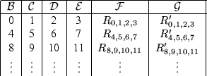 |
So that we can use a small fixed block size, we stripe blocks across
the partners using the erasure-correcting code. See
Figure 1 for an example block layout for a computer
![]() with 6 partners that is using
with 6 partners that is using ![]() and
and ![]() . We place
corresponding outputs of the erasure-correcting code on the same partner
(e.g.,
. We place
corresponding outputs of the erasure-correcting code on the same partner
(e.g., ![]() holds all the first redundancy blocks in
Figure 1) to make reconfiguration easier (see
Section 2.6).
holds all the first redundancy blocks in
Figure 1) to make reconfiguration easier (see
Section 2.6).
 |
Each computer decides for itself how to tradeoff reliability against
overhead by choosing values for ![]() and
and ![]() ; these choices in turn
determine the number of partners
; these choices in turn
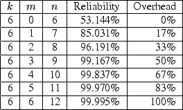
determine the number of partners ![]() it needs. To get a feel for
how these tradeoffs work in practice, see Figures 2
and 3. Figure 2 shows how reliability
rapidly and overhead slowly increase as the number of redundancy blocks
(
it needs. To get a feel for
how these tradeoffs work in practice, see Figures 2
and 3. Figure 2 shows how reliability
rapidly and overhead slowly increase as the number of redundancy blocks
(![]() ) is increased while holding the number of data blocks (
) is increased while holding the number of data blocks (![]() )
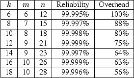
constant. Figure 3 shows that the overhead can be
decreased for a given level of reliability by increasing the number of
partners (
)
constant. Figure 3 shows that the overhead can be
decreased for a given level of reliability by increasing the number of
partners (![]() ). (Unlike traditional RAID systems, we can use
high values of
). (Unlike traditional RAID systems, we can use
high values of ![]() and
and ![]() because backup and restoration are relatively
insensitive to latency.)
because backup and restoration are relatively
insensitive to latency.)
These figures were calculated via the binomial distribution assuming that individual Internet computers fail independently and are 90% reliable. More precisely, they assume that when a computer tries to restore its data, the probability that a particular one of its partners still has its data, uncorrupted, and is sufficiently available during a limited restoration time window to supply that data is 90%.
This number is meant to be conservative; we expect from our personal experience that the real number will be considerably higher. Indeed, the only empirical study we know of on PC availability, Bolosky et al. [3], found that over half of all Microsoft's corporate desktops were up over 95% of the time when pinged hourly. As that study included some PCs that are shut down at night or over the weekend and a reasonable restoration window would probably be at least 24 hours, their numbers underestimate restoration availability for machines promising 24-hour availability. Nonetheless, even when using our conservative number, our calculations show that high reliability can be achieved with low overhead.
We expect randomly-chosen Internet PCs to fail independently except in cases of widespread virus damage, sustained loss of Internet connectivity, and (in the case of uncooperative environments) coordinated attacks involving multiple computers. See Section 3.3 for discussion of why we believe the later is unlikely to be a problem in practice.
 |