| ||||||||||||||||||||||||||||||||||||||||||||||||||||
|
USENIX 2002 Annual Technical Conference, Freenix Track - Paper
[USENIX 2002 Technical Program Index]
Gscope: A Visualization Tool for Time-Sensitive SoftwareAshvin Goel, Jonathan Walpole
AbstractThis paper describes gscope, a visualization tool for time-sensitive applications. Gscope provides an oscilloscope-like interface that can be integrated with applications. It focuses on software visualization and is thus designed to handle various types of signal waveforms, periodic or event-driven, in single or multi-threaded environments as well as local or distributed applications. Gscope helps in visually verifying system correctness and modifying system parameters and thus can complement standard debugging techniques and be used to build compelling software demos. Initial experiments with using gscope show that the library has low overhead.
1 IntroductionModern processor speeds and high speed networks have made multimedia and other timing-sensitive applications common on desktop computers. For instance, today a standard desktop computer comes equipped with a DVD player, DVD and CD burner, TV tuner and digital video editing and conferencing software, making it a full featured home audio and video client or server. Although these types of timing-sensitive applications are becoming common, implementing them is non-trivial because existing tools for visualizing and debugging alter the timing behavior. For instance, a standard debugger stops an application and thus affects its timing behavior. Current techniques for visualizing, testing and debugging time-sensitive applications involve some or all of these steps: 1) create an experimental setup, 2) generate data in real-time, 3) collect data and store it to files, 4) process the file data offline, and 5) plot the data. The first three steps are complicated by the fact that the programmer attempts to minimize the impact of these steps on the application's timing behavior. The programmer must often repeat these steps several times before being satisfied with the results. In addition, for a distributed application, data files must be collected from multiple machines and transferred to a single machine where the data is correlated before it can be processed.1 The problem with this approach is that the visualization and debugging cycle is long and error prone. It is error prone because the steps outlined above are often not an integral part of the application. Further, with this approach, it is not easy to demonstrate or experimentally validate system behavior in real-time. Unlike the ad hoc tools used for visualizing time-sensitive software, there exists a time-tested visualization tool in the hardware community: the oscilloscope. The invention of the oscilloscope started a revolution that allowed ``seeing'' sound and other signals, experiencing data, and gaining insights far beyond equations and tables [11]. Today, an oscilloscope, together with a logic analyzer, is used for several purposes such as debugging, testing and experimenting with various types of hardware that often have tight timing requirements. We believe a similar approach can be applied effectively for visualizing time-sensitive software systems. We have implemented a software visualization tool and library called gscope that borrows some of its ideas from an oscilloscope. The gscope design is motivated by the following goals:
Gscope focuses on visualization of time-sensitive software applications. It can be used for visualizing time-dependent variables such as network bandwidth, latency, jitter, fill levels of buffers in a pipeline, CPU utilization, etc. We have implemented gscope and have been using it for the last two years. We have used it for visualizing and debugging various time-sensitive applications, including a CPU scheduler [19], a quality-adaptive streaming media player [14], a network traffic generator called mxtraf [13], and various control algorithms such as a software implementation of a phase-lock loop [9]. We believe that applications using gscope will see a direct benefit in terms of reducing the visualizing, debugging and testing cycle time. Some of the key features of gscope are: support for multiple scopes and signals, dynamic addition and removal of scopes and signals, adjustment of program or control parameters, support for arbitrary signal types, time and frequency representation of signals, support for discrete-time and event-driven signals, support for distributed visualization, saving of signal data, replay of signal data, adjustment of per-signal parameters and scope parameters, and a programmatic interface for every action that can be performed from the GUI. These features help fulfill the many of the goals that motivated the design of gscope. In our experience, perhaps the most significant difference between the signals produced by software components and the signals typically visualized in an oscilloscope is the number of signal or event sources. Since software signals are not necessarily tied to specific pieces of hardware, applications can generate large numbers of disparate signals that need to be visualized and correlated. For instance, we use gscope to view dynamically changing process proportions as assigned by a CPU proportion-period scheduler [19]. Here, the number of signals depends on the number of running processes. As another example, since software signals are disconnected from hardware, they may be generated from remote sources (see Section 4.4). The remainder of this paper describes gscope in more detail. Section 2 explains the gscope design by describing the graphical components of gscope. Section 3 presents key components of the interface that enable an application to communicate with gscope. Section 4 discusses various aspects of programming the gscope library and it describes some of our experiences with gscope. Section 5 examines related work in this area and Section 6 presents future directions for Gscope. Finally, Section 7 presents our conclusions.
2 Graphical Interface
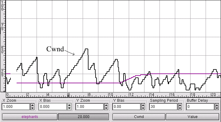
Gscope is a graphical library and thus its various features are best explained by briefly describing the visual components of the library. Then this section explains how we have used Gscope to visualize TCP behavior in an experimental network. Gscope has been implemented using the Gnome [6] and GTK [3] graphical toolkits. These GUI toolkits are multi-platform although they are primarily designed for the X Window System. They are free software and part of the GNU Project [18]. Both Gnome and GTK use the glib library that provides generic system functionality independent of the GUI. For instance, glib provides portable support for event sources, threads, and file and socket I/O. Gscope uses some of this glib functionality. The main graphical widget in the gscope library is called GtkScope, as shown in Figure 1. An application displays one or more signals by creating and passing a GtkScopeSig data structure for each signal to the library (see Section 3.1). The library creates a GtkScopeSignal object for each signal. Applications can create one or more GtkScope widgets. A screen shot of the GtkScope widget with the embedded canvas displaying two signals is shown in Figure 4. The zoom and bias widgets below the canvas allow scaling and translating the signal data. The sampling period widget allows changing the polling period of the displayed data. The delay widget allows setting the delay with which buffered signals are displayed on the scope (further described in Section 3.1). The x-axis ruler is sized in seconds and the y-axis ruler has a scale from 0 to 100.
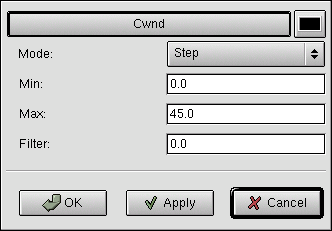
Under the zoom and bias widgets, signal parameters are displayed. Each signal has a signal name such as CWND and a Value button associated with it. Signal parameters, specified in the application using the GtkscopeSig data structure, can be modified by right clicking on the signal name, which brings up the window shown in Figure 2. Left clicking on the signal name toggles displaying the signal. When the Value button is pressed, the signal value is continuously displayed as shown with the CWND signal.
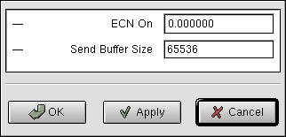
Gscope also allows storing, displaying and modifying application or control parameters that are application-wide and not specific to each GtkScope widget. Figure 3 shows an example of a control parameter window with two application parameters.
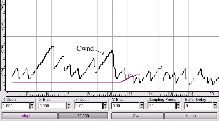
A Gscope ExampleThis section describes how the gscope library is used to visualize network behavior using the mxtraf network traffic generator application [13]. With Mxtraf, a small number of hosts can be used to saturate a network with a tunable mix of TCP and UDP traffic. The primary purpose of mxtraf is to allow stress testing of experimental networks. The experiment shown in Figures 4 and 5 compares the behavior of TCP and ECN [8](explicit congestion notification) flows in a congested wide-area network. To emulate a simple wide-area network, we use a Linux router between a client and a server machine and use nistnet [17] to add delay and bandwidth constraints at the router. In this experiment, we use mxtraf to generate varying number of long-lived flows (called elephants) that transfer data from the server to the client. Figures 4 and 5 show two signals each. The elephants signal shows the number of long-lived flows over time. This number is changed from 8 to 16 roughly half way through the x-axis. The CWND signal shows the TCP or ECN congestion window (at the server) of one (arbitrarily chosen) long-lived flow in Figures 4 and 5 respectively. This window provides an estimate of the short-term bandwidth achieved by the flow. These figures show how the window changes with a changing number of long-lived flows. While the absolute magnitude of the window is not very relevant in the short term period shown in the figures (since it changes dramatically over short intervals), one significant difference between the two flows is the number of timeouts experienced by each flow. Both TCP and ECN reduce the congestion window to one upon a timeout. The lowest value of the CWND signal in the graphs corresponds to a CWND value of one. The graphs show that while ECN does not hit this value, TCP hits it several times. Additional signals (not shown in the figures) confirm that there is a timeout each time CWND reaches one. Since timeouts affect TCP throughput and latency significantly, this experiment indicates that ECN can potentially improve flow throughput. We use mxtraf to dynamically change the number of different types of flows, switch between different TCP variants and visualize network behavior in real time. Such visualization has revealed several interesting properties (and bugs) in TCP behavior that would have been hard to determine otherwise. For instance, a TCP variant that we have implemented for low-latency TCP streaming [10] initially showed significant unexpected timeouts that we finally traced to an interaction with the SACK implementation.
3 Gscope APIThis section describes the interface data structures that enable an application to communicate with gscope. The gscope library The gscope interface is relatively simple but powerful. The gscope interface consists of three components: 1) signal specification, 2) control parameter specification for configuring the application and 3) tuple format for streaming, recording and viewing data.
3.1 Signal InterfaceGscope can acquire signal data from applications in one of two acquisition modes: polling or playback. In polling mode, signals are obtained from the running program using the signal interface described below. Polled signals can be unbuffered or buffered. In unbuffered mode, gscope polls and displays single sampling points. In buffered mode, applications enqueue signal samples with timestamps into a buffer and gscope displays these samples with a user-specified delay. The buffered mode enables applications to push data to the scope. For instance, an application can listen for kernel events on a netlink socket and push these event samples to the gscope buffer. Gscope polls the buffer periodically to display the samples. Polled signals can be displayed in the time or frequency domain. In addition, the polled data can be recorded to a file. Section 4 discusses the polling overhead and the finest polling granularity that is supported in gscope. In the playback mode, data is obtained from a file and displayed. This file format is described in Section 3.3. Both polling and playback modes have a polling period associated with them. In both modes, data is displayed one pixel apart each polling period (for the default zoom value). A signal is specified to the gscope library using a GtkScopeSig structure shown below:
The examples below show the GtkScopeSig specification for the elephants and CWND signals. The elephants signal consists of an integer value that will be sampled by gscope. The CWND signal uses the get_cwnd function to determine the CWND value of the socket fd.
3.1.0.1 Unbuffered SignalsFor unbuffered signals, the INTEGER, BOOLEAN, etc. field is sampled and displayed. of the union in the GtkScopeSigData structure depending on the type of the signal. When the signal type is FUNC, the function is invoked with the two arguments arg1 and arg2 (passed in by the user during GtkScopeSig initialization) and the function's return value is the value of the signal data. The function mechanism allows reading arbitrary signal data.
3.1.0.2 Buffered SignalsFor buffered signals, gscope reads data from a scope-wide buffer that has timestamped signal data in a tuple format (described in Section 3.3) and displays this data with a user-specified delay. Gscope provides applications an API for inserting the timestamped signal data in the buffer.
3.2 Control Parameter InterfaceApplication or control parameters as shown in Figure 3 can be read and modified by the gscope library using the GtkScopeParameter structure. These parameters are not displayed but generally used to modify application behavior. The GtkScopeParameter structure is very similar to the GtkScopeSig structure. However, while signals can only be read, application parameters can be read and written also.
3.3 Tuple FormatSignals can be streamed to gscope. For instance, streamed signals allow distributed visualization in real time. Signals can also be recorded to a file and gscope can replay signals from the file. In all these cases, signal data is delivered, generated or stored in a textual tuple format. Each tuple consists of three quantities: time, value and signal name. This format allows multiple signals to be delivered to gscope or recorded in the same file. As a special case, if there is only one signal, then the third quantity may not exist. In that case, signals are simply time-value tuples. When signals are streamed or replayed from a recorded file, the time field of successive tuples is in increasing time order and its value is in milliseconds. Data is displayed one pixel apart for each polling period (for the default zoom value). For instance, if the polling period is 50 ms, then data points in the file that are 100 ms apart will be displayed 2 pixels apart.
3.4 Programming With Gscope
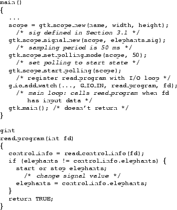
The Gscope library has a programmatic interface for every action that can be performed from the GUI. Figure 6 presents a fragment of a simple program that shows how the gscope library is used. After creating the scope, the elephants_sig signal (defined in Section 3.1) is added to scope and scope is set to polling mode, where it polls the value of elephants every 50 ms. The function that manipulates the elephants value is called read_program and it runs when the server has control data available from the client. In this usage style, the read_program function is I/O driven and performs non-blocking calls. Other ways of using the gscope library include 1) periodic invocation of read_program and 2) separation of the scope into its own thread. These issues are discussed further in Section 4.3.
4 DiscussionThe previous section has described the gscope API and how the gscope library can be used. This section discusses various aspects of programming the gscope library in more detail and it describes some of our experiences with gscope. Section 4.1 describes portability issues with the gscope library. Section 4.2 examines how gscope can be used for different types of signals effectively. Section 4.3 describes when it is appropriate to have a single-threaded or a multi-threaded gscope application, while Section 4.4 describes how data is polled and displayed from a distributed application. Section 4.5 describes the polling granularity in the current implementation and thus the type and range of applications that can be supported. Finally, Section 4.6 discusses the overhead of our approach.
4.1 Implementation PortabilityGscope has been implemented on the Linux OS and we have been using it for the last two years. Gscope can be installed on a vanilla Linux system that has Gnome software installed on it. Although, Gscope has not been ported to other free source operating systems such as BSD, we believe that the porting process should be simple since Gscope does not use any Linux specific functionality and Gnome has been ported to other OSs.
4.2 Signal TypesApplications often produce various types of signal data, such as clocked signals and event-driven signals. For instance, bandwidth monitoring can be done based on events that are packet arrivals. Gscope implements a discrete-time polling system but can also handle event-driven signal generation. Below, we describe various signal types and how gscope handles them.
4.3 Single vs. Multi-Threaded ApplicationsGscope is thread-safe and can be used by both single-threaded and multi-threaded applications. With multi-threaded applications, typically Gscope is run in its own thread while the application that is generating signals is run in a separate thread. This approach allows the gscope GUI to be scheduled independently of the application (unless gscope signals make application calls that need to acquire locks). However, it is the application thread's responsibility to acquire a global GTK lock if it needs to make gscope API calls. Single-threaded gscope applications must use event-driven programming. Such applications should either be periodic or they should be I/O driven and they should use non-blocking I/O system calls (since blocking calls would block the GUI as well). Periodic applications are supported directly by gscope. I/O driven applications can use the GTK GIOChannel functions to drive their events as shown in Figure 6. This approach allows all GUI and application events to be handled by the same event loop and does not require any locking. However, application logic can become more complex due to the use of non-blocking I/O system calls. We have implemented a single-threaded I/O driven gscope client-server library that is described in the next section.
4.4 Distributed ApplicationsGscope supports monitoring and visualization of distributed applications. It implements a single-threaded I/O driven client-server library that can be used by applications to monitor remote data. Clients use the gscope client API to connect to a server that uses the gscope server library. Clients asynchronously send BUFFER signal data in tuple format (described in Section 3.3) to the server. The server receives data from one or more clients asynchronously and buffers the data. It then displays these BUFFER signals to one or more scopes with a user-specified delay as described in Section 3.1. Data arriving at the server after this delay is not buffered but dropped immediately. Currently, we use the gscope client-server library in the mxtraf network traffic generator. The gscope client-server library allows visualizing and correlating client, server and network behavior (connections per second, connection errors per second, network throughput, latency, etc.) within a single scope.
4.5 Polling GranularityGscope uses the GTK timeout mechanism to implement polling. The default GTK timeout implementation uses the timeout feature of the POSIX select call. Although select allows specifying the timeout with a microsecond granularity, typically the kernel wakes processes at the granularity of the normal timer interrupt. The timer interrupt generally has a much coarser granularity. For instance, on Linux, this granularity is 10 ms. Thus gscope, which is implemented on Linux, is currently limited to this polling interval and has a maximum frequency is 100 Hz.2 In addition to coarse granularity timeouts, scheduling latencies in the kernel can induce loss in polling timeouts under heavy loads. To handle this problem, Gscope keeps track of lost timeouts and advances the scope refresh appropriately. Compared to an oscilloscope, Gscope has a much coarser polling granularity and thus relatively low bandwidth. For instance, the current Gscope implementation would not be appropriate for real-time low-delay display of a speech recognition application that monitors phone-line quality 8 KHz audio signals. Fortunately, in our experience, many software applications don't have tight polling requirements. Coarse granularity polling works well for three reasons: 1) many software applications have coarse time scales, 2) debugging software applications often only requires visualizing the long term trends of the signal, 3) many applications generate event-driven signals that are handled by techniques such as buffering or event aggregation as explained in Section 4.2. For instance, the audio signal could be read from the audio device and buffered by an application and gscope can display the signal with some delay using buffered signals. In our experience, the 10 ms polling granularity and loss of polling timeouts has not been a limiting factor for the gscope applications that we have implemented. However, Section 6 describes some directions for improving the polling granularity.
4.6 Scope OverheadWe measured the overhead of using the gscope library by running a simple application that polls and displays several different integer values. To measure overhead, we use a CPU load program that runs in a tight loop at a low priority and measures the number of loop iterations it can perform at any given period. The ratio of the iteration count when running gscope versus on an idle system gives an estimate of the gscope overhead. The gscope CPU overhead on a 600 MHz Pentium III processor is less than two percent while polling at 10 ms granularity (smallest granularity supported by the system) and less than one percent at 50 ms granularity. The increase in overhead with increasing number of signals being displayed ranges from 0.02 to 0.05 percent per signal. When compared to the number of signals displayed, polling granularity has a much larger effect on CPU consumption.
5 Related WorkThis section provides some background on oscilloscopes and compares them with gscope. Then it describes some oscilloscope-like applications that have been developed in the free software community. The oscilloscope is essentially a graph-displaying device - it draws a graph of an electrical signal. Oscilloscopes can help determine various signal properties: time and voltage values of a signal, frequency of an oscillating signal, phase difference between two oscillating signals, a malfunctioning component that is distorting the signal, AC and DC components of a signal and noise in a signal. Oscilloscopes put significant effort on visualization of repeating waveforms. For instance, they have trigger controls that help stabilize such waveforms. Oscilloscopes can be analog or digital. Analog oscilloscopes are preferred when it is important to display rapidly varying signals in ``real time''. However, digital oscilloscopes allow capture and viewing of events that may happen only once. They can process the digital waveform data or send the data to a computer for processing. Like gscope, they can store the digital waveform data for later viewing and printing and they also allow event aggregation. Gscope is similar in functionality to gstripchart [12], the Gnome stripchart program, that charts various user-specified parameters as a function of time such as CPU load and network traffic levels. The gstripchart program periodically reads data from a file, extracts a value and displays these values. However, unlike Gscope, gstripchart has a configuration file based interface rather than a programmatic interface, which limits its use for debugging or modifying system behavior. There is large body of work related to implementing software digital oscilloscope functionality for audio visualization. The basic idea is to record sound with a microphone and then display the digitized sound waves. Xoscope [20] is one such program. Xmms [4] displays sound frequency during audio playback. Baudline [2] is a real-time signal analysis tool and an offline time-frequency browser. These programs emulate the functionality of a digital oscilloscope much more closely than gscope. However, these programs are focusing on audio visualization while gscope focuses on visualization and debugging of software behavior. Thus certain oscilloscope features are not appropriate for gscope and vice-versa. There are hundreds of measurement tools that can be used for capturing system and network performance [1]. Gscope complements them because it can be used to visualize their output in real-time.
6 Future WorkWe expect to see more integration of oscilloscope functionality in gscope. Gscope currently does not have support for repeating waveforms. Thus, many oscilloscope features such as triggers that stabilize repeating waveforms or waveform envelop generation are not implemented in gscope. Gscope does not currently support printing of recorded data. Also, it does not have bindings for languages other than C. There are several options for supporting applications with more stringent polling requirements. First, Linux exposes the real-time clock on the Intel x86 processor that can generate interrupts at a maximum frequency of 8KHz. Unfortunately, this clock is exposed only to processes with root privileges and can only be used by one application at a time. Further, it is not clear how this mechanism can be used together with the GTK polling or event handling mechanism. The benefit of using the GTK polling mechanism is that all events, GUI as well as application events, are handled by the same mechanism and this allows implementing fully event-driven applications. Such an implementation is the norm for GUI applications [16,7].3 A second option is to improve the granularity of select in the kernel by connecting it to a more general fine-grained timing facility, such as soft-timers [5]. Improving the granularity of select will automatically help to improve the granularity of the GTK polling mechanism. Finally, kernel scheduling latencies can be reduced by using a preemptive kernel [15].
7 ConclusionsGscope is designed for visualizing time-sensitive software applications. Its goal is to reduce the cycle time needed for visualizing, testing and debugging time-sensitive applications by providing an oscilloscope-like interface that can be integrated with the application. In this paper, we have described the design and interface of the gscope library, presented some simple examples of using the library and then discussed various aspects related to programming the library. We have used gscope successfully in many of our applications and have built several compelling demos of our research work using this library. Gscope is free software. More information about gscope is available at https://gscope.sf.net.
Bibliography
Footnotes
|
|
This paper was originally published in the Proceedings of the FREENIX Track: 2002 USENIX Annual Technical Conference, June 10-15, 2002, Monterey Conference Center, Monterey, California, USA.
Last changed: 16 May 2002 ml |
|