Jian Zhang
SRI International Menlo Park, CA 94025
Phillip Porras
SRI International Menlo Park, CA 94025
Johannes Ullrich
SANS Institute Bethesda, MD 20814
A network address blacklist represents a collection of source IP addresses that have been deemed undesirable, where typically these addresses have been involved in some previous illicit activities. For example, DShield (a large-scale security-log sharing system) regularly compiles and posts a firewall-parsable blacklist of the most prolific attack sources seen by its contributors [17]. With more than 1700 contributing sources providing a daily stream of 30 million security log entries, such daily blacklists provide an informative view of those class C subnets that are among the bane of the Internet with respect to unwanted traffic. We refer to the blacklists that are formulated by a large-scale alert repository and consist of the most prolific sources in the repository's collection of data as the global worst offender list (GWOL). Another strategy for formulating network address blacklists is for an individual network to create a local blacklist based entirely on its own history of incoming communications. Such lists are often culled from a network's private firewall log or local IDS alert store, and incorporate the most repetitive addresses that appear within the logs. We call this blacklist scheme the local worst offender list (LWOL) method.
The GWOL and LWOL strategies have both strengths and inherent weaknesses. For example, while GWOLs provide networks with important information about highly prolific attack sources, they also have the potential to exhaust the subscribers' firewall filter sets with addresses that will simply never be encountered. Among the sources that do target the subscriber, GWOLs may miss a significant number of attacks, in particular when the attack sources prefer to choose their targets more strategically, focusing on a few known vulnerable networks [4]. Such attackers are not necessarily very prolific and are hence elusive to GWOLs. The sources on an LWOL have repetitively sent unwanted communications to the local network and are likely to continue doing so. However, LWOLs are limited by being entirely reactive - they only capture attackers that have been pounding the local network and hence cannot provide a potential for the blacklist consumer to learn of attack sources before these sources reach their networks.
Furthermore, both types of lists suffer from the fact that an attack source does not achieve candidacy until it has produced a sufficient mass of communications. That is, although it is desirable for firewall filters to include an attacker's address before it has saturated the network, neither GWOL nor LWOL offer a solution that can provide such timely filters. This is a problem particularly with GWOL. Even after an attacker has produced significant illicit traffic, it may not show up as a prolific source within the security log repository, because the data contributors of the repository are a very small set of networks on the Internet. Even repositories such as DShield that receive nearly 1 billion log entries per month represent only a small sampling of Internet activity. Significant attacker sources may elude incorporation into a blacklist until they have achieved extensive saturation across the Internet.
In summary, a high-quality blacklist that fortifies network firewalls should achieve high hit rate, should incorporate addresses in a timely fashion, and should proactively include addresses even when they have not been encountered previously by the blacklist consumer's network. Toward this goal, we present a new blacklist generation system which we refer to as the highly predictive blacklisting (HPB) system. The system incorporates 1) an automated log prefiltering phase to remove unreliable alert contents, 2) a novel relevance-based attack source ranking phase in which attack sources are prioritized on a per-contributor basis, and 3) a severity analysis phase in which attacker priorities are adjusted to favor attackers whose alerts mirror known malware propagation patterns. The system constructs final individualized blacklists for each DShield contributor by a weighted fusion of the relevance and severity scores.
HPB's underlying relevance-based ranking scheme represents a significant departure from the long-standing LWOL and GWOL strategies. Specifically, the HPB scheme examines not just how many targets a source address has attacked, but also which targets it has attacked. In the relevance-based ranking phase, each source address is ranked according to how closely related the source is to the target blacklist subscriber. This relevance measure is based on the attack source similarity patterns that are computed across all members of the DShield contributor pool (i.e., the amount of attacker overlap observed between the contributors). Using a data correlation strategy similar to hyper-text link analysis, such as Google's PageRank [2], the relationships among all the contributors are iteratively explored to compute an individual relevance value from each attacker to each contributor.
We evaluated our HPB system using more than 720 million log entries produced by DShield contributors from October to November 2007. We contrast the performance of the system with that of the corresponding GWOLs and LWOLs, using identical time windows, input data, and blacklist lengths. Our results show that for most contributors (more than 80%), our blacklist entries exhibit significantly higher hit counts over a multiday testing window than both GWOL and LWOL. Further experiments show that our scheme can proactively incorporate attacker addresses into the blacklist before these addresses reach the blacklist consumer network, and it can do so in a timely fashion. Finally, our experiments demonstrate that the hit count increase is consistent over time, and the advantages of our blacklist remain stable across various list lengths and testing windows.
The contribution of this paper is the introduction of the highly predictive blacklisting system, which includes our methodology for prefiltering, relevance-based ranking, attacker severity ranking, and final blacklist construction. Ours is the first exploration of a link-analysis-based scheme in the context of security filter production and to quantify the predictive quality of the resulting data. The HPB system is also one of the only new approaches we are aware of for large-scale blacklist publication that has been proposed in many years. However, our HPB system is applicable only to those users who participate as active contributors to collaborative security log data centers. Rather than a detriment, we hope that this fact provides some operators a tangible incentive to participate in security log contributor pools. Finally, the system discussed in this paper, while still a research prototype, has been fully implemented and deployed for nearly a year as a free service on the Internet at DShield.org. Our experience to date leads us to believe that this approach is both scalable and feasible for daily use.
The rest of the paper is organized as follows. Section 2 provides a background on previous work in blacklist generation and related topics. In Section 3 we provide a detailed description of the Highly Predictive Blacklist system. In Section 4 we present a performance evaluation of HPBs, GWOLs, and LWOLS, including assessments of the extent to which the above three desired blacklist properties (hit rate, proactive appearance, and timely inclusion) are realized by these three blacklists. In Section 5 we present a prototype implementation of the HPB system that is freely available to DShield.org log contributors, and we summarize our key findings in Section 6.
More agile forms of network blacklisting have also been explored, with the intention of rapidly publishing perimeter filters to control actively spreading malware epidemics [12,1,3,14]. For example, in [14] a peer-to-peer blacklisting scheme is proposed, where each network incorporates an address into its local blacklist when a threshold number of peers have reported attacks from this address. We separate our HPB system from these malware defense schemes. While the HPB system does incorporate a malware-oriented attacker severity metric into its final blacklist selection, we have not contemplated nor propose HPBs for use in the context of dynamic quarantine defenses for malware epidemics.
One key insight that inspired the HPB relevance-based ranking scheme was raised by Katti et al. [10], who identified the existence of stable correlations among the attackers reported by security log contributors. Here we introduce a relevance-based recommendation scheme that selects candidate attack sources based on the attacker overlaps found among peer contributors. This relevance-based ranking scheme can be viewed as a random walk on the correlation graph, going from one node to another following the edges in the graph with the probability proportional to the weight of the graph. This form of random walk has been applied in link-analysis systems such as Google's PageRank [2], where it is used to estimate the probability that a webpage may be visited. Similar link analysis has been used to rank movies [13] and reading lists [19].
The problem of predicting attackers has also been recently considered in [24] using a Guassian process model. However, [24] purely focused on developing statistical learning techniques for attacker prediction based on collaborative filtering. In this paper, we present a comprehensive blacklisting generation system that considers many other characteristics of attackers. The prediction part is only one component in our system. Furthermore, the prediction model presented here is completely different from the one in [24] (Gaussian process model in [24] and link analysis model here). By taking some penalty in predictive power, the prediction model presented here is much more scalable, which is of necessity for implementing a deployable service (Section 5).
Finally, [23] provides a six-page summary of the earliest release of our DShield HPB service, including a high-level description of an early ranking scheme. In this paper we have substantially expanded this algorithm and present its full description for the first time. This present paper also introduces the integration of metrics to capture attack source maliciousness in its final rank selection, and presents the full blacklist construction system. We also present our quantitative evaluation of multiple system properties, and address several open questions that have been raised over the past year since our initial prototype.
We illustrate our blacklisting system in Figure 1. The system constructs blacklists in three stages. First, the security alerts supplied by sensors across the Internet are preprocessed. This removes known noises in the alert collection. We call this the prefiltering stage. The preprocessed data are then fed into two parallel engines. One ranks, for each contributors, the attack sources according to their relevance to that contributor. The other scores the sources using a severity assessment that measures their maliciousness. The relevance ranking and the severity score are combined at the last stage to generate a final blacklist for each contributor.
We descibe the prefiltering process in Section 3.1, relevance ranking in Section 3.2, severity score in Section 3.3 and the final production of the blacklists in Section 3.4.
As a preliminary step prior to blacklist construction, we apply three filtering techniques to the DShield alert logs. First, the HPB system removes from consideration DShield logs produced from attack sources from invalid or unassigned IP address space. Here we employ the bogon list created by the Cymru team that captures addresses that are reserved, not yet allocated, or delegated by the Internet Assigned Number Authority [16]. Typically, such addresses should not be routed, but otherwise do appear anyway in the DShield data. In addition, reserved addresses such as the 10.x.x.x or 192.168.x.x may also appear in misconfigured contributor logs that are not useful for translating into blacklists.
Second, the system prefilters from consideration network addresses from Internet measurement services, web crawlers, or common software update sources. From experience, we have developed a whitelist of highly common sources that, while innocuous from an intrusion perspective, often generate alarms in DShield contributor logs.
Finally, the HPB system applies heuristics to avoid common false positives that arise from commonly timed-out network services. Specifically, we exclude logs produced from source ports TCP 53 (DNS), 25 (SMTP), 80 (HTTP), and 443 (often used for secure web, IMAP, and VPN), and from destination ports TCP 53 (DNS) and 25 (SMTP). Firewalls will commonly time out sessions from these services when the server or client becomes unresponsive or is slow. In practice, the combination of these prefiltering steps provides approximately a 10% reduction in the DShield input stream prior delivery to the blacklist generation system.
Our notion of attacker relevance is a measure that indicates how close the attacker is related to a particular blacklist consumer. It also reflects the likelihood to which the attacker may come to the blacklist consumer in the near future. Note that this relevance is orthogonal to metrics that measure the severity (or benignness) of the source, which we will discuss in the next section.
In our context, the blacklist consumers are the contributors that supply security logs to a log-sharing repository such as DShield. Recent research has observed the existence of attacker overlap correlations between DShield contributors [10], i.e., there are pairs of contributors that share quite a few common attackers, where the common attacker is defined as a source address that both contributors have logged and reported to the repository. This research also found that this attacker overlap phenomenon is not due to attacks that select targets randomly (as in a random scan case). The correlations are long lived and some of them are independent of address proximity. We exploit these overlap relationships to measure attacker relevance.
We first illustrate a simple concept of attacker relevance.
Consider a collection
of security logs displayed in a tabular form as shown in Table 1. We use the rows of the table to represent
attack sources and the columns to represent contributors. We refer to
the unique source addresses that are reported within the log
repository as attackers, and use the terms ``attacker'' and
``source'' interchangeably. Since the
contributors are also the targets
of the logged attacks, we refer to them as victims. We will use
the terms ``contributor'' and ``victim'' interchangeably. An asterisk
``*'' in the table cell indicates that the corresponding source has
reportedly attacked the corresponding contributor.
Let us assume that Table 1 represents a series of logs contributed
in the recent past by our five victims, ![]() through
through ![]() . Now suppose we would
like to calculate the relevance of the sources for contributor
. Now suppose we would
like to calculate the relevance of the sources for contributor ![]() based on
these attack patterns. From the attack table we observe that contributors
based on
these attack patterns. From the attack table we observe that contributors
![]() and
and ![]() share multiple common attackers.
share multiple common attackers. ![]() also shares one common attack
source (
also shares one common attack
source (![]() ) with
) with ![]() , but does not share attacker overlap with the other contributors.
Given this observation, between sources
, but does not share attacker overlap with the other contributors.
Given this observation, between sources ![]() and
and ![]() , we would say
that
, we would say
that ![]() has more relevance to
has more relevance to ![]() than
than ![]() because
because
![]() has reportedly attacked
has reportedly attacked ![]() , which has recently
experienced multiple attack source
overlaps with
, which has recently
experienced multiple attack source
overlaps with ![]() . But the victims of
. But the victims of ![]() 's attacks share no
overlap with
's attacks share no
overlap with ![]() .
Note that this relevance measure is quite different from
the measures based on how prolific the attack source has been. The latter would
favor
.
Note that this relevance measure is quite different from
the measures based on how prolific the attack source has been. The latter would
favor ![]() over
over ![]() , as
, as ![]() has attacked more victims than
has attacked more victims than ![]() . In this sense,
which contributors a source has attacked is of greater significance to our scheme
than how many victims it has attacked. Similarly, between
. In this sense,
which contributors a source has attacked is of greater significance to our scheme
than how many victims it has attacked. Similarly, between ![]() and
and ![]() ,
, ![]() is more
relevant, because the victim of
is more
relevant, because the victim of ![]() (
(![]() ) shares more common attacks with
) shares more common attacks with
![]() than the victim of
than the victim of ![]() (
(![]() ). Finally, because
). Finally, because ![]() has
attacked both
has
attacked both ![]() and
and ![]() , we would like to say that it is the
most relevant among
, we would like to say that it is the
most relevant among ![]() , and
, and ![]() .
.
To formalize the above intuition, we model the attack correlation
relationship between contributors using a correlation graph, which
is a weighted undirected graph ![]() . The nodes in the
graph consist of the contributors
. The nodes in the
graph consist of the contributors
![]() . There is an
edge between node
. There is an
edge between node ![]() and
and ![]() if
if ![]() is correlated with
is correlated with ![]() . The
weight on the edge is
determined by the strength of the correlation (i.e., occurrences of attacker
overlap) between the two
corresponding contributors.
We now introduce some notation for the relevance model.
. The
weight on the edge is
determined by the strength of the correlation (i.e., occurrences of attacker
overlap) between the two
corresponding contributors.
We now introduce some notation for the relevance model.
Let ![]() be the number of
nodes (number of contributors) in the correlation graph. We use
be the number of
nodes (number of contributors) in the correlation graph. We use
![]() to denote the adjacency matrix of the correlation graph, where the
entry
to denote the adjacency matrix of the correlation graph, where the
entry
![]() in this matrix is the weight of the edge
between node
in this matrix is the weight of the edge
between node ![]() and
and ![]() . For a source
. For a source ![]() , we denote by
, we denote by ![]() the set of contributors that have reported an attack from
the set of contributors that have reported an attack from ![]() .
.
![]() can be written in a vector form
can be written in a vector form
![]() such that
such that ![]() if
if ![]() and
and ![]() otherwise. We also associate with each source
otherwise. We also associate with each source ![]() a relevance
vector
a relevance
vector
![]() such
that
such
that ![]() is the relevance value of attacker
is the relevance value of attacker ![]() with respect to
contributor
with respect to
contributor ![]() . We use lowercase boldface to indicate vectors and uppercase
boldface to indicate matrices. Table 2 summarizes our notation.
. We use lowercase boldface to indicate vectors and uppercase
boldface to indicate matrices. Table 2 summarizes our notation.
We now describe how to derive the matrix ![]() from the
attack reports.
Consider the following two cases. In Case 1, contributor
from the
attack reports.
Consider the following two cases. In Case 1, contributor ![]() sees attacks from 500 sources and
sees attacks from 500 sources and ![]() sees 10 sources. Five of these
sources attack both
sees 10 sources. Five of these
sources attack both ![]() and
and ![]() . In Case 2, there are also
five common sources. However,
. In Case 2, there are also
five common sources. However, ![]() sees only 50 sources and
sees only 50 sources and ![]() sees
10. Although the number of overlapping sources is the same (i.e., 5 common sources),
the strength of connection between
sees
10. Although the number of overlapping sources is the same (i.e., 5 common sources),
the strength of connection between ![]() and
and ![]() is different
in the two cases. If a contributor observes a lot of attacks,
it is expected that there should be more
overlap between this contributor and the others. Let
is different
in the two cases. If a contributor observes a lot of attacks,
it is expected that there should be more
overlap between this contributor and the others. Let ![]() be the
number of sources seen by
be the
number of sources seen by ![]() ,
, ![]() the number seen by
the number seen by ![]() , and
, and
![]() the number of common attack sources. The ratio
the number of common attack sources. The ratio
![]() shows
how important
shows
how important ![]() is for
is for ![]() while
while
![]() shows how important
shows how important
![]() is for
is for ![]() . Since we want
. Since we want
![]() to reflect the
strength of the connection between
to reflect the
strength of the connection between ![]() and
and ![]() ,
we set
,
we set
![]() .
One may view this new
.
One may view this new ![]() as a standardized correlation
matrix. Figure 2
shows the matrix
as a standardized correlation
matrix. Figure 2
shows the matrix ![]() for Table 1 constructed using this method.
for Table 1 constructed using this method.
Given this correlation matrix, we follow the aforementioned intuition
and calculate the relevance as
![]() . This is to say that
if the repository reports that source
. This is to say that
if the repository reports that source ![]() has attacked contributor
has attacked contributor ![]() ,
this fact contributes a value of
,
this fact contributes a value of
![]() to the source's relevance with respect to the victim
to the source's relevance with respect to the victim ![]() .
Written in vector form, it gives us
.
Written in vector form, it gives us
The above simple relevance calculation lacks certain desired properties. For example, the simple relevance value is calculated solely from the observed activities from the source by the repository contributors. In some cases, this observation does not represent the complete view of the source's activity. One reason is that the contributors consist of only a very small set of networks in the Internet. Before an attacker saturates the Internet with malicious activity, it is often the case that only a few contributors have observed the attacker. The attacker may be at its early stage or it has attacked many places, most of which do not participate in the security log sharing system. Therefore, one may want a relevance measure that has a ``look-ahead'' capability. That is, the relevance calculation should take into consideration possible future observations of the source and include these anticipated observations from the contributors into the relevance values.
Figure 3 gives an example where one may apply this
``look-ahead'' feature. (Examples here are independent
of the one shown in Table 1.) The correlation graph of
Figure 3 consists of four contributors numbered 1,
2, 3, and 4. Contributor 2 reported an attack from source ![]() (represented by the star). Our goal is to evaluate how relevant this
attacker is to contributor 1 (double-circled node). Using Equation 1, the relevance
would be zero. However, we observe that
(represented by the star). Our goal is to evaluate how relevant this
attacker is to contributor 1 (double-circled node). Using Equation 1, the relevance
would be zero. However, we observe that ![]() has relevance
0.5 with respect to contributor 3 and relevance 0.3 with respect to
contributor 4. Although at this time, contributors 3 and 4 have not
observed
has relevance
0.5 with respect to contributor 3 and relevance 0.3 with respect to
contributor 4. Although at this time, contributors 3 and 4 have not
observed ![]() yet, there may be possible future attacks from
yet, there may be possible future attacks from ![]() . In
anticipation of this, when evaluating
. In
anticipation of this, when evaluating ![]() 's relevance with respect to
contributor 1, contributors 3 and 4 pass to contributor 1 their
relevance values after multiplying them with the weights on their
edges, respectively. The attacker's relevance value for
contributor 1 then is 0.5*0.2+0.3*0.2 = 0.16. Note that, had
's relevance with respect to
contributor 1, contributors 3 and 4 pass to contributor 1 their
relevance values after multiplying them with the weights on their
edges, respectively. The attacker's relevance value for
contributor 1 then is 0.5*0.2+0.3*0.2 = 0.16. Note that, had ![]() actually attacked contributors 3 and 4, the contributors would have
passed the relevance value 1 (again after multiplying them with the
weights on the edges) to contributor 1.
actually attacked contributors 3 and 4, the contributors would have
passed the relevance value 1 (again after multiplying them with the
weights on the edges) to contributor 1.
This can be viewed as a relevance propagation process. If a
contributor ![]() observed an attacker, we say that the attacker has an
initial relevance value 1 for that contributor. Following the edges that go
out of the contributor, a fraction of this relevance can be
distributed to the neighbors of the contributor in the graph. Each of
observed an attacker, we say that the attacker has an
initial relevance value 1 for that contributor. Following the edges that go
out of the contributor, a fraction of this relevance can be
distributed to the neighbors of the contributor in the graph. Each of
![]() 's neighbors receives a share of relevance that is proportional
to the weight on the edge that connects the neighbor to
's neighbors receives a share of relevance that is proportional
to the weight on the edge that connects the neighbor to
![]() . Suppose
. Suppose ![]() is one of the neighbors.
A fraction of the relevance received by
is one of the neighbors.
A fraction of the relevance received by ![]() is then further
distributed, in similar fashion, to its neighbors. The propagation
of relevance continues until the relevance values for each contributor
reach a stable state.
is then further
distributed, in similar fashion, to its neighbors. The propagation
of relevance continues until the relevance values for each contributor
reach a stable state.
This relevance propagation process has another benefit besides the
``look-ahead'' feature. Consider the correlation
graph given in Figure 4 (a). The subgraph formed
by nodes 1, 2, 3, and 4 is very different from that formed by nodes
1, 5, 6, and 7. The subgraph from nodes 1, 2, 3, and 4 is well
connected (in fact it forms a clique). The contributors in the
subgraph are thus more tied together. We call them a correlated
group. (We use a dotted circle to indicate the
correlated group in Figure 4.) There may be
certain intrinsic similarities between the members in the correlated
group (e.g., IP address proximity, similar vulnerability). Therefore,
it is natural to assign more relevance to source addresses that have
attacked other contributors in the same correlated group. For example,
consider the sources ![]() and
and ![]() in Figure 4.
They both attacked three contributors. All the edges in the correlation
graph have the same weights. (Hence, we omitted the weights in the
figure.) We would like to say that
in Figure 4.
They both attacked three contributors. All the edges in the correlation
graph have the same weights. (Hence, we omitted the weights in the
figure.) We would like to say that ![]() is more relevant than
is more relevant than ![]() for
contributor 1. If we calculate the relevance value by
Equation 1, the values would be the same for the two
attackers. Relevance propagation helps to give more value to the
attacker
for
contributor 1. If we calculate the relevance value by
Equation 1, the values would be the same for the two
attackers. Relevance propagation helps to give more value to the
attacker ![]() because members of the correlated group are well
connected. There are more paths in the subgraph that lead from the
contributors where the attack happened to the contributor for which we
are evaluating the attacker relevance. For example, the relevance
from contributor 2 can propagate to contributor 3 and then to contributor 1.
It can also go to contributor 4 and then to contributor 1. This is effectively
the same as having an edge with larger weight between the contributors 2
and 1. Therefore, relevance propagation can effectively discover and
adapt to the structures in the correlation graph. The relevance values
assigned then reflect certain intrinsic relationships among
contributors.
because members of the correlated group are well
connected. There are more paths in the subgraph that lead from the
contributors where the attack happened to the contributor for which we
are evaluating the attacker relevance. For example, the relevance
from contributor 2 can propagate to contributor 3 and then to contributor 1.
It can also go to contributor 4 and then to contributor 1. This is effectively
the same as having an edge with larger weight between the contributors 2
and 1. Therefore, relevance propagation can effectively discover and
adapt to the structures in the correlation graph. The relevance values
assigned then reflect certain intrinsic relationships among
contributors.
We extend Equation 1 to employ relevance
propagation. If we propagate the relevance values to the immediate
neighbors in the correlation graph, we obtain a relevance vector
![]() that represents the propagated values. Now we propagate
the relevance values one more hop. This gives us
that represents the propagated values. Now we propagate
the relevance values one more hop. This gives us
![]() . The relevance vector that reflects the total relevance
value each contributor receives is then
. The relevance vector that reflects the total relevance
value each contributor receives is then
![]() . If we let the propagation process
iterate indefinitely, the relevance vector would become
. If we let the propagation process
iterate indefinitely, the relevance vector would become
![]() . There is a
technical detail in this process we need to resolve. Naturally,
we would like the relevance value to decay along the path of
propagation. The further it goes on the graph, the smaller its
contribution becomes. To achieve this, we scale the matrix
. There is a
technical detail in this process we need to resolve. Naturally,
we would like the relevance value to decay along the path of
propagation. The further it goes on the graph, the smaller its
contribution becomes. To achieve this, we scale the matrix
![]() by a constant
by a constant ![]() such that the 2-norm
of the new matrix
such that the 2-norm
of the new matrix
![]() becomes smaller than
one. With this modification, an attacker will have only a negligible
relevance value to contributors that are far away in the correlation
graph. Putting the above together, we compute the relevance vector by
the following equation:
becomes smaller than
one. With this modification, an attacker will have only a negligible
relevance value to contributors that are far away in the correlation
graph. Putting the above together, we compute the relevance vector by
the following equation:
We observe that
![]() is the solution for
is the solution for ![]() in the following system of linear equations:
in the following system of linear equations:
Equation 3 can be solved to give
![]() , where
, where ![]() is the identity matrix. Also, since
is the identity matrix. Also, since
![]() ,
,
![]() . This
gives the relevance vector for each attack source. The
sources are then ranked, for each contributor, according to the
relevance values. As each attack source
has a potentially different relevance value for each contributor, the rank
of a source with respect to different contributors is different.
Note that our concept of relevance measure and relevance propagation does
not depend on a particular choice of the
. This
gives the relevance vector for each attack source. The
sources are then ranked, for each contributor, according to the
relevance values. As each attack source
has a potentially different relevance value for each contributor, the rank
of a source with respect to different contributors is different.
Note that our concept of relevance measure and relevance propagation does
not depend on a particular choice of the ![]() matrix. As long as
matrix. As long as
![]() reflects the connection weight between the contributors,
our relevance measure applies.
reflects the connection weight between the contributors,
our relevance measure applies.
We now consider the problem of measuring the degree to which each attack source exhibits known patterns of malicious behavior. In the next section, we will disuss how this measure can be fused into our final blacklist construction decisions. In this section we will describe our model of malicious behavior and the attributes we extract to map each attacker's log production patterns to this model.
Our model of malicious behavior, in this instance, focuses on identifying typical scan-and-infect malicious software (or malware). We define our malware behavior pattern as that of an attacker who conducts an IP sweep to small sets of ports that are known to be associated with malware propagation or backdoor access. This behavior pattern matches the malware behavior pattern documented by Yegeneswaren et.al. in [20], as well as our own most recent experiences (within the last twelve months) of more than 20K live malware infections observed within our honeynet [21]. Other potential malware behavior patterns may be applied, for example, such as the scan-oriented malicious address detection schemes outlined in the context of dynamic signature generation [11] and malicious port scan analysis [9]. Regardless of the malware behavior model used, the design and integration of other severity metrics into the final blacklist generation process can be carried out in a similar fashion.
For the set of log entries over the relevance-calculation time window, we calculate several attributes for each attacker's /24 network address. (Our blacklists are specified on a per /24 basis, meaning that a single malicious address has the potential to induce a LAN-wide filter. This is standard practice for DShield and other blacklists.) For each attacker, we assign a score to target ports associated with the attacker, assigning a different weight depending on whether or not the port is associated with known malware communications.
Let ![]() be the set of malware-associated ports, where we
currently uses the definition in Figure 5.
This
be the set of malware-associated ports, where we
currently uses the definition in Figure 5.
This ![]() is derived from various AV lists and our honeynet
experiences. We do not argue that this list is complete and can be
expanded across the life of our HPB service. However, our experiences
in live malware analysis indicate that the entries in
is derived from various AV lists and our honeynet
experiences. We do not argue that this list is complete and can be
expanded across the life of our HPB service. However, our experiences
in live malware analysis indicate that the entries in ![]() are both
highly common and highly indicative of malware propagation.
are both
highly common and highly indicative of malware propagation.
Let the number of target ports that attacker ![]() connects to
be
connects to
be ![]() , and the total number of unique ports
connected to be defined as
, and the total number of unique ports
connected to be defined as ![]() . We associate a weighting (or importance)
factor
. We associate a weighting (or importance)
factor ![]() for all ports in
for all ports in ![]() , and a weighting factor
, and a weighting factor ![]() for all
nonmalware ports. We then compute a malware port score (
for all
nonmalware ports. We then compute a malware port score (![]() ) metric
for each attacker as follows:
) metric
for each attacker as follows:
Here, we intend ![]() to be of greater weight than
to be of greater weight than ![]() , and choose an
initial default of
, and choose an
initial default of
![]() .
. ![]() has the property that even if
a large
has the property that even if
a large ![]() is found, if
is found, if ![]() is also large (as in a horizontal portscan),
then
is also large (as in a horizontal portscan),
then ![]() will remain small. Again, our intention is to promote a malware
behavior pattern in which malware propagation will tend to target fewer
specific ports, and is not associated with attackers that engage in
horizontal port sweeps.
will remain small. Again, our intention is to promote a malware
behavior pattern in which malware propagation will tend to target fewer
specific ports, and is not associated with attackers that engage in
horizontal port sweeps.
Next, we compute the set of unique target IP addresses connected
to by attacker ![]() . We refer to this count as
. We refer to this count as ![]() . A large
. A large ![]() represents confirmed IP sweep behavior, which we strongly associate
with our malware behavior model.
represents confirmed IP sweep behavior, which we strongly associate
with our malware behavior model. ![]() is the exclusive
prioritization metric used by GWOL, whereas here we consider
is the exclusive
prioritization metric used by GWOL, whereas here we consider ![]() a
secondary factor to
a
secondary factor to ![]() in computing a final malware behavior score.
We could also include metrics regarding the number of DShield sensors
(i.e., unique contributor IDs) that have reported the attacker, which
arguably represents the degree of consensus in the contributor
pool that the attack source is active across the Internet. However,
the IP sweep pattern is of high interest, even when the
IP sweep experiences may have been reported only by a smaller set of
sensors.
in computing a final malware behavior score.
We could also include metrics regarding the number of DShield sensors
(i.e., unique contributor IDs) that have reported the attacker, which
arguably represents the degree of consensus in the contributor
pool that the attack source is active across the Internet. However,
the IP sweep pattern is of high interest, even when the
IP sweep experiences may have been reported only by a smaller set of
sensors.
Third, we compute an optional tertiary behavior metric that captures
the ratio of national to international addresses that are targeted by
attacker ![]() . Within the DShield repository we find many
cases of sources (such as from China, Russian, the Czech Republic) that
exclusively target international victims. However, this may also
illustrate a weakness in the DShield contributor pool, as there may be
very few contributors that operate sensors within these countries. We
incorporate a dampening factor
. Within the DShield repository we find many
cases of sources (such as from China, Russian, the Czech Republic) that
exclusively target international victims. However, this may also
illustrate a weakness in the DShield contributor pool, as there may be
very few contributors that operate sensors within these countries. We
incorporate a dampening factor ![]() (
(
![]() ) that
allows the consumer to express the degree to which the
) that
allows the consumer to express the degree to which the ![]() factor should
be nullified in computing the final severity score for each attacker.
factor should
be nullified in computing the final severity score for each attacker.
Finally, we compute a malware severity score ![]() for each candidate
attacker that may appear in the set of final blacklist entries:
for each candidate
attacker that may appear in the set of final blacklist entries:
The three factors are computed in order of significance in mapping
to our malware behavior model. Logarithm is used because in our model,
the secondary metric (![]() ) and the tertiary metric (
) and the tertiary metric (![]() ) are less
important than the malware port score and we only care about their order
of magnitude.
) are less
important than the malware port score and we only care about their order
of magnitude.
For each attacker, we now have both its relevance ranking and its severity score. We can combine them to generate a final blacklist for each contributor.
For the final blacklist, we would like to include the attackers
that have strong relevance and discard the nonrelevant attackers.
To generate a final list of length ![]() , we use the attacker's
relevance ranking to compile a candidate list of size
, we use the attacker's
relevance ranking to compile a candidate list of size ![]() . (We
often set
. (We
often set ![]() .)
Then, we use severity scores of the attackers on the candidate list
to adjust its ranking and pick the
.)
Then, we use severity scores of the attackers on the candidate list
to adjust its ranking and pick the ![]() highest-ranked attackers
to form the final list. Intuitively, the adjustment should promote
the rank of an attacker if the severity assessment indicates that it
is very malicious. Toward this goal, we define a final
score that combines the attacker's relevance rank in the candidate list
and its severity assessment.
In particular, let
highest-ranked attackers
to form the final list. Intuitively, the adjustment should promote
the rank of an attacker if the severity assessment indicates that it
is very malicious. Toward this goal, we define a final
score that combines the attacker's relevance rank in the candidate list
and its severity assessment.
In particular, let ![]() be the relevance rank of the attacker
be the relevance rank of the attacker ![]() (i.e.,
(i.e.,
![]() is the k-th entry in the candidate list). Recall from last section
is the k-th entry in the candidate list). Recall from last section
![]() is the severity score of
is the severity score of ![]() . The final score
. The final score ![]() is defined
to be
is defined
to be
![]() promotes the rank of an attacker according
to its maliciousness. The larger the value of
promotes the rank of an attacker according
to its maliciousness. The larger the value of ![]() is, the more
the attacker is moved above comparing to its original rank.
A
is, the more
the attacker is moved above comparing to its original rank.
A ![]() of value 1 would then
move the attacker above for one half of the size of the final list comparing
to its original rank.
The ``S'' shaped
of value 1 would then
move the attacker above for one half of the size of the final list comparing
to its original rank.
The ``S'' shaped ![]() transforms
the severity assessment
transforms
the severity assessment ![]() into a value between 0 and 1. The
less-malicious attackers often give an assessment score below 3. After
transformation, they will receive only small promotions. On the other
hand, malicious attackers that give an assessment score above 7 will
be highly promoted.
into a value between 0 and 1. The
less-malicious attackers often give an assessment score below 3. After
transformation, they will receive only small promotions. On the other
hand, malicious attackers that give an assessment score above 7 will
be highly promoted.
To generate the final list, we sort the ![]() values of
the attackers in the candidate list and then pick
values of
the attackers in the candidate list and then pick ![]() of them that
have the smallest
of them that
have the smallest ![]() .
.
We created an experimental HPB blacklist formulation system. To evaluate the HPBs, we performed a battery of experiments using the DShield.org security firewall and IDS log repository. We examined a collection of more than 720 million log entries produced by DShield contributors from October to November 2007. Since our relevance measure is based on correlations between contributors, HPB production is not applicable to contributors that have submitted very few reports (DShield has contributors that hand-select or sporadically contribute logs, providing very few alerts). We therefore exclude those contributors that we find effectively have no correlation with the wider contributor pool or simply have too few alerts to produce meaningful results. For this analysis, we found that we could compute correlation relationships for about 700 contributors, or 41% of the DShield contributor pool.
To assess the performance of the HPB system, we compare its performance relative to the standard DShield-produced GWOL [17]. In addition, we compare our HPB performance to that of LWOLs, which we compute individually for all contributors in our comparison set. For the purpose of our comparative assessment, we fixed the length of all three competing blacklists to exactly 1000 entries. However, after we present our comparative performance results, we will then continue our investigation by analyzing how the blacklist length affects the performance of the HPBs.
In the experiments, we generate GWOL, LWOL, and HPBs using data for a certain time period and then test the blacklists on data from the time window following this period. We call the period used for producing blacklists the training window and the period for testing the prediction window. In practice, the training period represents a snapshot of the most recent history of the repository, used to formulate each blacklist for a contributor that is then expected to use the blacklist for the length of the prediction window. The sizes of these two windows are not necessarily equal. We will first describe experiments that use 5-day lengths for both the training window and the prediction window. We then present experiments that investigate the effects of the two windows' lengths on HPB quality.
DShield logs submitted during the prediction window are used to determine how many sources included within a contributor's HPB are indeed encountered during that prediction window. We call this value the blacklist hit count. We view each blacklist address filter not encountered by the blacklist consumer as an opportunity cost to have prevented the deployment of other filters that could have otherwise blocked unwanted traffic. In this sense, we view our hit count metric as an important measure of the effectiveness of a blacklist formulation algorithm. Note that our HPBs are formulated with severity analysis while the other lists are not. As the severity analysis prefers malicious activities, we expect that the hits on the HPBs are more malicious.
To compare the three types of lists,
we take 60 days of data, divided
into twelve 5-day windows. We repeat the experiment 11 times using the
![]() -th window as the training window and the
-th window as the training window and the ![]() -th window as
the testing window. In the training window, we construct HPB,
LWOL, and GWOL. Then the three types of lists are tested on the
data in the testing window.
-th window as
the testing window. In the training window, we construct HPB,
LWOL, and GWOL. Then the three types of lists are tested on the
data in the testing window.
Table 3 shows the total number of hits summed over the contributors for HPB, GWOL, and LWOL, respectively. It also shows the ratio of HPB hits over that of GWOL and LWOL. We see that in every window, HPB has more hits than GWOL and LWOL. Overall, HPBs predict 20-30% more hits than LWOL and GWOL. Note that there are quite large variances among the number of hits between time windows. Most of the variances, however, are not from our blacklist construction, rather they are from the variance among the number of attackers the networks experience in different testing windows.
The results in Table 3 show HPB's hit improvement over time windows. We now investigate the distribution of the HPB's hit improvement across contributors in one time window. We use two quantities for comparison. The first is the hit count improvement, which is simply the HPB hit count minus the hit count of the other list. The second comparative measure we used is the relative hit count improvement (RI), which is the ratio in percentage of the HPB hit count increase over the other blacklist hit count. If the other list hit count is zero we define RI to be 100x the HPB hit count, and if both hit counts are zero we set RI to 100.
Table 5 provides a summary of hit-count improvement for the 200 contributors where HPBs perform the best. The hit-count results for all the contributors are summarized in Table 4.
Figure 7 compares HPB to GWOL. The left panel of the
figure plots the histogram showing the distribution of the hit improvement
across the contributors. The x-axis indicates improvements, and the
hight of the bars
represents the number of contributors whose improvement fall in the
corresponding bin. Bars left to ![]() represent contributors for whom the
HPB has worse performance and bars on the right represent contributors
for whom HPBs performed better. For most contributors, the
improvment is positive. The largest improvement reaches 732. For only
a few contributors, HPB performs worse in this time window.
represent contributors for whom the
HPB has worse performance and bars on the right represent contributors
for whom HPBs performed better. For most contributors, the
improvment is positive. The largest improvement reaches 732. For only
a few contributors, HPB performs worse in this time window.
The panel on the right of Figure 7 plots the RI (ratio % of HPB's hit count increase over GWOL's hit count) distribution. We sort the RI values and plot them against the contributors. We label the x-axis by cummulative percentage, i.e., a tick on x-axis represents the percentage of contributors that lie to the left of the tick. For example, the tick 20 means 20 percent of the contributors lie left to this tick. There are contributors for which the RI value can be more than 3900. Instead of showing such large RI values, we cut off the plot at RI value 300. From the plot, we see that there are about 20% of contributors for which the HPBs achieve an RI more than 100, i.e., the HPB at least doubled the GWOL hit count. For about half of the contributors, the HPBs have about 25% more hits (an RI of 25). The HPBs have more hits than GWOL for almost 90% of the contributors. Only for a few contributors (about 7%), HPBs perform worse. (We discuss the reasons why HPB may perform worse in Section 4.4.)
Figure 8 compares HPB hit counts to those of LWOL. The data are plotted in the same way as in Figure 7. Overall, HPBs demonstrate a performance advantage over LWOL. The IV and RI values also exhibit similar distributions. However, comparing Figures 8 and 7, we see that HPB has more hit improvement comparing to LWOL than to GWOL in this time window.
One clear motivating assumption in secure collaborative defense strategies is that participants have the potential to prepare themselves from attacks that they have not yet encountered. We will say that a new attack occurs when a contributor produces a DShield log entry from a source that this contributor has never before reported. In this experiment, we show that HPB analysis provides contributors a potential to predict more new attacks than GWOL. (LWOL is not considered, since by definition it includes only attackers that are actively hitting the LWOL owner.) For each contributor, we construct two new HPB and GWOL lists with equal length of 1000 entries, such that no entries have been reported by the contributor during our training window. We call these lists HPB-local (HPB minus local) and GWOL-local (GWOL minus local), respectively. Figure 9 compares HPB-local and GWOL-local on their ability to predict on new attack sources for the local contributor. These hit number plots demonstrate that HPB-local provides substantial improvement over the predictive value of GWOL.
By timely inclusion, we refer to the ability of a blacklist to incorporate addresses relevant to the blacklist owner before those addresses have saturated the Internet. To investigate the timeliness of the GWOL, LWOL, and the HPB we examine how many contributors need to report a particular attacker before it can be included into the respective blacklists. We focus our attention on the set of attackers within these blacklists that did carry out attacks during the prediction window. And we use the number of distinct victims (contributors) that a source attacked in the training window to measure the extent to which the source has saturated the Internet. Figure 10 plots the distribution of the number of distinct victims across different attackers on the three blacklists. As expected, the attackers that get selected on the GWOL were the most prolific in the training period. In particular, all the sources on the GWOL have attacked more than 20 contributors and almost 1/3 of them attacked more than 200 contributors. To some extent, these attackers have saturated the Internet with their activities. (DShield sensors are a very small sample of the Internet. A random attacker has to target many places to be picked up by the sensors.) The LWOLs select attacker addresses that focused on the local networks. Most of these addresses had attacked far fewer contributors. HPBs's distribution is close to that of the LWOL, hence allowing the incorporation of attackers that have not saturated the Internet.
The results in the above experiments show that the HPB provides an increase in hit count performance across the majority of all contributors. We now ask the following question: is the HPB's performance consistent for a given contributor over time? In this experiment, we investigate this consistency question.
We use a 60-day DShield dataset. We divide it into 12 time
windows,
![]() . We generate blacklists from data in
time window
. We generate blacklists from data in
time window ![]() and test the lists on data in
and test the lists on data in ![]() . For each
contributor
. For each
contributor ![]() , we compare HPB with GWOL and obtain eleven improvement values
for window
, we compare HPB with GWOL and obtain eleven improvement values
for window ![]() to
to ![]() . We denote them
. We denote them
![]() . We then define a consistency index (CI)
for each contributor. If
. We then define a consistency index (CI)
for each contributor. If ![]() , we say that the HPB performs
well for
, we say that the HPB performs
well for ![]() in window
in window ![]() . Otherwise, we say that the HPB performs worse.
CI is the difference between the number of
windows in which HPB performs well and the ones in which HPB performs
poorly, i.e.,
. Otherwise, we say that the HPB performs worse.
CI is the difference between the number of
windows in which HPB performs well and the ones in which HPB performs
poorly, i.e.,
![]() .
If HPB consistently performs better than GWOL for a contributor,
its
.
If HPB consistently performs better than GWOL for a contributor,
its ![]() should be close to 11. If it consistently performs worse,
the
should be close to 11. If it consistently performs worse,
the ![]() value will be close to -11. However, if the HPB performance
flip-flops, its CI value will be close to zero.
Figure 11 plots the sorted
CI values against the contributors.
(Again, we label the x-axis by cummulative percentage.)
We see that for almost
70% of the contributors, HPB's performance is extremely consistent.
They all have a CI value of 11, meaning
for the eleven time windows, the HPB always predicts more hits for them than
GWOL. For more than 90% of the contributors, HPBs demonstrate fairly
good consistency. With few contributors does the performance
switch back and forth. Only 5 contributors show performance index below -3.
value will be close to -11. However, if the HPB performance
flip-flops, its CI value will be close to zero.
Figure 11 plots the sorted
CI values against the contributors.
(Again, we label the x-axis by cummulative percentage.)
We see that for almost
70% of the contributors, HPB's performance is extremely consistent.
They all have a CI value of 11, meaning
for the eleven time windows, the HPB always predicts more hits for them than
GWOL. For more than 90% of the contributors, HPBs demonstrate fairly
good consistency. With few contributors does the performance
switch back and forth. Only 5 contributors show performance index below -3.
The consistency investigation sheds some light on the reason why there is a small percentage of contributors for which the HPBs (sometimes) perform worse than the other list. HPB construction is based on the relevance measure. The relevance relates attack sources to contributors according to the past security logs collected by the repository. If a contributor has relatively stable correlations (stable for several days) with other contributors or it experiences stable attack patterns, the relevance measure can capture this and thus produce blacklists with more hits. Such HPBs will also be consistent in hit-count performance. On the other hand, if the correlation is not stable or the attacks exhibit few patterns, the relevance measure will be less effective and may produce blacklists with fewer hits. Such HPBs will not be consistent in performance because sometimes they may guess right and produce more hits and sometimes they may guess wrong.
This can be seen in Figure 11. All the consistent HPBs have CI value 11. These HPBs have both consistency and better hit-count performance. There is no HPB that shows CI value -11. HPB never performs consistently worse.
This is particularly useful because the consistency of an HPB's performance can be used to indicate whether the HPB user (the contributor) has stable correlations. If so, HPBs can be better blacklists to use. The experiment result suggests that most of the contributors have stable correlations. In practice, given a few cycles of computing HPB and GWOL for a DShield contributor, we can provide an informed recommendation as to which list that contributor should adopt over a longer term.
In this experiment, we vary the length of the blacklists to be 500, 1000, 5000 and 10000. We then compare the hit counts of HPBs, GWOLs, and LWOLs. Because in all the experiments, the improvements for different contributors display similar distributions, we will simply plot the medians of the hit rates of these respective blacklists. (Hit rate is the hit count divided by the blacklist length.) Our results are illustrated in Figure 12, and show that HPBs have the hit rate advantage for all these choices in blacklist length. The relative amount of advantage is also maintained across different lengths.
Although the hit rate for the shorter lists is higher, the number of hits are larger for the longer lists. This is so for all three types of blacklists. It shows that the longer the list is, the more entries on the list are wasted (in the sense that they do not get hit). Therefore, it may not always be desirable to use very long lists.
We now investigate how far into the future the HPB can maintain its
advantage over GWOL and LWOL, and how different training window sizes
affect an HPB's hit count. The former helps to determine how often we
need to recompute the blacklist, and the latter helps to select the
right amount of history data as the input to our system. The left
panel of Figure 13 shows the median of the hit count
of HPB, GWOL, and LWOL on day
![]() for each
individual day in the prediction window. All lists are generated
using data from a 5-day window prior to the prediction window.
For all blacklists, the number of hits decreases along time. The
HPB maintains an advantage over the entire duration of the
prediction window. From this plot, we also see that the blacklists need
to be refreshed frequently. In particular, there may be an almost 30%
hit drop when the HPB is more than a week old.
for each
individual day in the prediction window. All lists are generated
using data from a 5-day window prior to the prediction window.
For all blacklists, the number of hits decreases along time. The
HPB maintains an advantage over the entire duration of the
prediction window. From this plot, we also see that the blacklists need
to be refreshed frequently. In particular, there may be an almost 30%
hit drop when the HPB is more than a week old.
The right panel of Figure 13 plots hit-number medians for four HPBs. These HPBs are generated in a slightly different way from the HPBs we used so far. In previous experiments, to generate an HPB, we produce the correlation matrix from a set of attack reports. Then the sources in the same set of reports are selected into HPBs based on their relevance. In this experiment, we construct the correlation matrix using reports from training windows of size 2, 5, 7, and 10 days. Then the sources that are in the reports within the 5-day window right before the prediction (test) window are picked based on their relevance. In this formulation, we exclude sources that appear only in reports from distant history; we view their extended silence to represent a significant loss in relevance. The remainder of the test is performed in the same way as the previous experiments, i.e., the hit counts are obtained in the following 5-day prediction window. The experiment result shows that there is a slight increase in the hit counts going from a 2-day training window to a 5-day training window. The hit counts then remain roughly the same for the other training-window size. This indicates that for most of the contributors, the correlation matrix can be quite stable over time.
In mid 2007, we deployed an initial prototype implementation of the HPB system, providing a subset of the features described in this paper. This initial deployment was packaged as a free Internet blacklisting service for DShield log contributors [22,23]. HPB blacklists are constructed for all contributors daily, and each contributor can download her individual HPB through her DShield website account. To date, we have had a relative small pool of HPB downloaders (roughly 70 users over the most 3 months). We now describe several aspects of fielding a practical and scalable implementation of an HPB system based on our initial deployment experiences. We present an assessment of the algorithm complexity, the DShield service implementation, and discuss some open questions raised from the open release of our service.
Because HPBs are constructed from a relatively high-volume corpus of
security logs, our system must be prepared to process well over
100M log entries per day to process entries over the current 5-day
training window. The bottleneck of the system is the relevance ranking.
Therefore, our complexity discussion focuses on the ranking algorithm.
There is always an amount of complexity that
is linear to the size of the alert data. That is, let ![]() be
the number of alerts in the data collection; we have a minimum
complexity of
be
the number of alerts in the data collection; we have a minimum
complexity of ![]() . Our discussion will focus on other
complexities incurred by the algorithm besides this linear-time
requirement.
. Our discussion will focus on other
complexities incurred by the algorithm besides this linear-time
requirement.
We denote by ![]() and
and ![]() the number of sources in the data
collection and the number of contributors to the repository
respectively. In practice, one can expect
the number of sources in the data
collection and the number of contributors to the repository
respectively. In practice, one can expect ![]() to be in the order of
thousands while
to be in the order of
thousands while ![]() is much larger, typically in the tens of
millions. We obtain
is much larger, typically in the tens of
millions. We obtain ![]() and
and ![]() by going through
the repository and doing simple accounting. The adjacency matrix
by going through
the repository and doing simple accounting. The adjacency matrix
![]() requires the most work to construct. To obtain this
matrix, we record every overlapped attack while going through the
alert data and then perform standardization. The latter steps require
us to go through the whole matrix, which results in
requires the most work to construct. To obtain this
matrix, we record every overlapped attack while going through the
alert data and then perform standardization. The latter steps require
us to go through the whole matrix, which results in ![]() complexity.
complexity.
Besides going through the data, the most time-consuming step in the
relevance estimate process is the computation that solves the linear
equations in Equation 3. At first glance, because
for each source ![]() , we have a linear system determined by Equation 3, it seems that we need to solve
, we have a linear system determined by Equation 3, it seems that we need to solve ![]() linear
systems. This can be expensive as
linear
systems. This can be expensive as ![]() is very large. Further
investigation shows that while
is very large. Further
investigation shows that while ![]() is different per source
is different per source
![]() , the
, the
![]() part of the solution to Equation 3 is the same for all
part of the solution to Equation 3 is the same for all ![]() . Therefore, we need to
compute it only once, which requires
. Therefore, we need to
compute it only once, which requires ![]() time by brute force
or
time by brute force
or
![]() using more sophisticated
methods [5]. Because
using more sophisticated
methods [5]. Because ![]() is sparse, once we have
is sparse, once we have
![]() , the total time to obtain the ranking
scores for all the sources and all the contributors is
, the total time to obtain the ranking
scores for all the sources and all the contributors is
![]() . Assuming
. Assuming ![]() is much smaller than
is much smaller than ![]() , the total
complexity to make relevance ranking is
, the total
complexity to make relevance ranking is
![]() . For a data set that contains a billion records contributed
by a thousand sensors, generating a thousand rankings requires only
several trillion operations (additions and multiplications). This can
be easily handled by modern computers. In fact, in our experiments,
with
. For a data set that contains a billion records contributed
by a thousand sensors, generating a thousand rankings requires only
several trillion operations (additions and multiplications). This can
be easily handled by modern computers. In fact, in our experiments,
with ![]() in the high tens of millions and
in the high tens of millions and ![]() on the order of one
thousand, it takes less than 30 minutes to generate all contributor
blacklists on an Intel Xeon 3.6 GHz machine.
on the order of one
thousand, it takes less than 30 minutes to generate all contributor
blacklists on an Intel Xeon 3.6 GHz machine.
The pragmatics of deploying an HPB service through the DShield website are straightforward. DShield log contributors are already provided private web accounts in order to review their reports. However, to ease the automatic retrieval of HPBs, users are not required to log in via DShield's standard web account procedure. Instead, contributors wishing to access their individual HPBs can create account-specific hexadecimal tokens, and can then append this token to the HPB URL. This token has a number of advantages, particularly for developing and maintaining automated HPB retrieval scripts. That is, a user account password may be changed regularly, but the retrieval token (and script) will remain unaffected.
To provide further protection of the integrity and confidentiality of an HPB the user may also pull the HPB via https. A detached PGP signature can be retrieved in case https is not available or not considered a sufficient proof of authenticity.
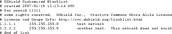
HPBs are distributed using a simple tab-delimited format. The first column identifies the network address. The second column provides the netmask. Additional columns are used to provide more information about the respective offender, such as the name of the network and country of origin (or type of attacks seen). These additional columns are intended for human review of the HPB. Comments may be added to the blocklist. All comments start with a # mark. A sample blocklist is shown in Figure 14.
As we have made efforts to implement, test, and advertise early versions of the HPB system, several open questions have been raised regarding the ability of adversaries to game the HPB system. That is, can an attacker contribute data to DShield with the intention of manipulating HPB production in ways that negatively harm HPB quality? Let us consider several questions that arise from the fact that HPBs are derived from volunteer sources, which may include dishonest contributors that are actively trying to harm or negatively manipulate HPB results.
Can an attacker cause a consumer to incorporate an unsuspecting
victim address into a third party's HPB? Let us assume that attacker
![]() participates as one or more DShield contributors (
participates as one or more DShield contributors (![]() might
register multiple IDs) and knows that consumer
might
register multiple IDs) and knows that consumer ![]() is also a DShield
contributor and an active HPB user. Furthermore,
is also a DShield
contributor and an active HPB user. Furthermore, ![]() would like to
cause address
would like to
cause address ![]() to be inserted into consumer
to be inserted into consumer ![]() 's HPB. There are
two potential strategies
's HPB. There are
two potential strategies ![]() can pursue to achieve this goal. First,
can pursue to achieve this goal. First,
![]() can spoof attacks as address
can spoof attacks as address ![]() , directing these attacks to other
contributors that are highly correlated with
, directing these attacks to other
contributors that are highly correlated with ![]() . However,
. However, ![]() 's
correlated contributor set is neither readily available to
's
correlated contributor set is neither readily available to ![]() (unless
(unless
![]() is a DShield insider) or necessarily stable over time.
More plausibly,
is a DShield insider) or necessarily stable over time.
More plausibly, ![]() could artificially cause his own contributor IDs to
report the same attacks as
could artificially cause his own contributor IDs to
report the same attacks as ![]() . He can do this by attacking
. He can do this by attacking ![]() with
a set of spoofed addresses, and then reporting similarly spoofed logs
from his contributor IDs. Once a sufficient set of attack logs with
identical spoofed attackers is reported by
with
a set of spoofed addresses, and then reporting similarly spoofed logs
from his contributor IDs. Once a sufficient set of attack logs with
identical spoofed attackers is reported by ![]() and
and ![]() ,
, ![]() could then
positively influence the likelihood that address
could then
positively influence the likelihood that address ![]() will be inserted
into
will be inserted
into ![]() 's HPB. While this is a
possible threat, we also observe that similar attacks can be
launched against GWOL and more trivially against LWOL.
Furthermore, in the case of GWOL,
's HPB. While this is a
possible threat, we also observe that similar attacks can be
launched against GWOL and more trivially against LWOL.
Furthermore, in the case of GWOL, ![]() will be inserted in all
consumers' GWOLs, whereas A must launch this attack individually
against each HPB consumer.
will be inserted in all
consumers' GWOLs, whereas A must launch this attack individually
against each HPB consumer.
Can an attacker cause his own address to be excluded from a
specific third-party HPB? Let us assume that ![]() would like to
guarantee that address
would like to
guarantee that address ![]() will not appear in
will not appear in ![]() 's HPB. This is very
difficult for
's HPB. This is very
difficult for ![]() to guarantee. While
to guarantee. While ![]() may cause artificial
alignment between his and
may cause artificial
alignment between his and ![]() 's logs using the alert spoofing method
discussed above,
's logs using the alert spoofing method
discussed above, ![]() cannot control what other addresses may also
align with
cannot control what other addresses may also
align with ![]() . If
. If ![]() attacks other contributors that are aligned
with
attacks other contributors that are aligned
with ![]() ,
, ![]() has the potential to enter
has the potential to enter ![]() 's HPB.
's HPB.
Can an attacker fully prevent or poison all HPB production? In short, yes. Data poisoning is a fundamental threat that arises in all volunteer contributor-based data centers, and is an inherently difficult threat to overcome. However, DShield does occasionally experience, and incorporate countermeasures for issues such as accidental flooding and sensor misconfiguration. DDoS threats also arise and are dealt with by DShield case by case.
HPB generation could also be specifically targeted by a malicious contributor
that attempts to artificially inflate the number of attacker or victim
addresses, which will increase the values of ![]() or
or ![]() , as described
in our complexity analysis, Section 5.1. However, to
sufficiently prohibit HPB production, the contributor would
necessarily produce highly anomalous volumes of attackers (or sources)
that would likely allow us to identify and (temporarily) filter this
contributor.
, as described
in our complexity analysis, Section 5.1. However, to
sufficiently prohibit HPB production, the contributor would
necessarily produce highly anomalous volumes of attackers (or sources)
that would likely allow us to identify and (temporarily) filter this
contributor.
In this paper, we introduced a new system to generate blacklists for contributors to a large-scale security-log sharing infrastructure. The system employs a link analysis method similar to Google's PageRank for blacklist formulation. It also integrates substantive log prefiltering and a severity metric that captures the degree to which an attacker's alert patterns match those of common malware-propagation behavior. Experimenting on a large corpus of real DShield data, we demonstrate that our blacklists have higher attacker hit rates, better new attacker prediction quality, and long-term performance stability.
In April of 2007, we released a highly predictive blacklist service at DShield.org. We view this service as a first experimental step toward a new direction of high-quality blacklist generation. We also believe that this service offers a new argument to help motivate the field of secure collaborative data sharing. In particular, it demonstrates that people who collaborate in blacklist formulation can share a greater understanding of attack source histories, and thereby derive more informed filtering policies. As future work, we will continue to evolve the HPB blacklisting system as our experience grows through managing the blacklist service.
![\includegraphics[width=5in,height=1.5in]{figs/sys.eps}](img1.png)
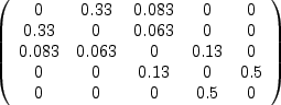
![\includegraphics[width=2.5in,height=1.5in]{figs/prop1b.eps}](img44.png)
![\includegraphics[width=5in,height=1.6in]{figs/prop2b.eps}](img45.png)
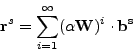
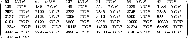
![\includegraphics[width=2.5in,height=1.6in]{figs/phi.eps}](img92.png)
![\includegraphics[width=5in,height=1.6in]{figs/gvp.eps}](img97.png)
![\includegraphics[width=5in,height=1.6in]{figs/lvp.eps}](img98.png)
![\includegraphics[width=5in,height=1.6in]{figs/pred.eps}](img100.png)
![\includegraphics[width=2.5in,height=1.6in]{figs/sat.eps}](img101.png)
![\includegraphics[width=2.5in,height=1.6in]{figs/cons.eps}](img112.png)
![\includegraphics[width=2.5in,height=1.6in]{figs/bl_len.eps}](img113.png)
![\includegraphics[width=5in,height=1.6in]{figs/tpws.eps}](img114.png)