We had initially thought that a policy targeting the necessary number
of non-idle cycles would result in good behavior, but the previous
example highlights why we use the speed-setting policies described in
§4.3. We used the same
![]() scheduler
proposed by Govil [6] and Pering [5]
and also examined by
Pering et al. in [5]; Perings later paper
in [11] did not examine scheduler heuristics and only
used real-time scheduling with application-specified scheduling goals.
scheduler
proposed by Govil [6] and Pering [5]
and also examined by
Pering et al. in [5]; Perings later paper
in [11] did not examine scheduler heuristics and only
used real-time scheduling with application-specified scheduling goals.
Our findings indicate
that the
![]() algorithm can not settle on the clock speed
that maximizes CPU utilization. Although a given set of parameters can
result in optimal performance for a single application, these tuned
parameters will probably not work for other applications, or even the
same application with different input. The variance inherent in many
deadline-based applications prevents an accurate assessment of the
computational needs of an application. The
algorithm can not settle on the clock speed
that maximizes CPU utilization. Although a given set of parameters can
result in optimal performance for a single application, these tuned
parameters will probably not work for other applications, or even the
same application with different input. The variance inherent in many
deadline-based applications prevents an accurate assessment of the
computational needs of an application. The
![]() policy can be
easily designed to ensure that very few deadlines will be missed, but
this results in minimal energy savings. We use an MPEG player as a
running example in this section, as it best exemplifies behavior that
illustrates the multitude of problems in past-based interval
algorithms. Our intuition is that if there's is a single application
that illustrates simple, easy-to-predict behavior, it should be
MPEG. Our measurements showed that the MPEG application can run at
132MHz without dropping frames and still maintain synchronization
between the audio and video. An ideal clock scheduling policy would
therefore
target a speed of 132MHz.
policy can be
easily designed to ensure that very few deadlines will be missed, but
this results in minimal energy savings. We use an MPEG player as a
running example in this section, as it best exemplifies behavior that
illustrates the multitude of problems in past-based interval
algorithms. Our intuition is that if there's is a single application
that illustrates simple, easy-to-predict behavior, it should be
MPEG. Our measurements showed that the MPEG application can run at
132MHz without dropping frames and still maintain synchronization
between the audio and video. An ideal clock scheduling policy would
therefore
target a speed of 132MHz.
However, without information from the user level application, a kernel cannot accurately determine what deadlines an application operates under. First, an application may have different deadline requirements depending on its input; for example, an MPEG player displaying a movie at 30fps has a shorter deadline than one running at 15fps. Although the deadlines for an application with a given input may be regular, the computation required in each deadline interval can vary widely. Again, MPEG players demonstrate this behavior; I-frames (key or reference) require much more computation than P-frames (predicted), and do not necessarily occur at predictable intervals.
One method of dealing with this variance is to look at lengthy
intervals which will, by averaging, reduce the variance of the
computational observations. Our utilization plots showed that even
using 100ms intervals, significant variance is exhibited. In addition
to interval length, the number of intervals over which we average
(![]() ) of the
) of the
![]() policy can also be manipulated. We conducted a
comprehensive study and varied the value of
policy can also be manipulated. We conducted a
comprehensive study and varied the value of ![]() from 0 (the PAST
policy) to 10 with each combination of the speed-setting policies
(i.e. using ``peg'' to set the CPU speed to the highest point,
or ``one'' to increment or decrement the speed).
from 0 (the PAST
policy) to 10 with each combination of the speed-setting policies
(i.e. using ``peg'' to set the CPU speed to the highest point,
or ``one'' to increment or decrement the speed).
Our conclusions from the results with our benchmarks is that the
weighted average has undesirable behavior. The number of intervals
not only represents the length of interval to be considered; it
also represents the
lag before the system responds, much like the simple averaging
example described above. Unlike that simple policy, once
![]() starts responding, it will do so quickly. For example, consider a
system using an mechanism with an upper boundary of 70%
utilization and ``one'' as the algorithms used to increment or
decrement the clock speed. Starting from an idle state, the clock will
not scale to 206MHz for 120 ms (12 quanta). Once it scales up,
the system will continue to do so (as the average utilization will
remain above 70%) unless the next quantum is partially idle. This
occurs because the previous history is still considered with equal
weight even when the system is running at a new clock value.
starts responding, it will do so quickly. For example, consider a
system using an mechanism with an upper boundary of 70%
utilization and ``one'' as the algorithms used to increment or
decrement the clock speed. Starting from an idle state, the clock will
not scale to 206MHz for 120 ms (12 quanta). Once it scales up,
the system will continue to do so (as the average utilization will
remain above 70%) unless the next quantum is partially idle. This
occurs because the previous history is still considered with equal
weight even when the system is running at a new clock value.
The boundary conditions used by Pering in [5] result in a system that scales more rapidly down than up. Table 1 illustrates how this occurs. If the weighted average is 70%, a fully active quantum will only increase the average to 73% while a fully idle quantum will reduce it to 63% - thus, there is a tendency to reduce the processor speed.
The job of the scheduler is made even more difficult by applications that attempt to make their own scheduling decisions. For example, the default MPEG player in the Itsy software distribution uses a heuristic to decide whether it should sleep before computing the next frame. If the rendering of a frame completes and the time until that frame is needed is less than 12ms, the player enters a spin loop; if it is greater than 12ms, the player relinquishes the processor by sleeping. Therefore, if the player is well ahead of schedule, it will show significant idle times; once the clock is scaled close to the optimal value to complete the necessary work, the work seemingly increases. The kernel has no method of determining that this is wasteful work.
Furthermore, there is some mathematical justification for our assertion that
![]() fundamentally exhibits undesirable behavior, and will not
stabilize on an optimal clock speed, even for simple and predictable workloads.
Our analysis only examines the ``smoothing'' portion of
fundamentally exhibits undesirable behavior, and will not
stabilize on an optimal clock speed, even for simple and predictable workloads.
Our analysis only examines the ``smoothing'' portion of
![]() , not the
clock setting policy. Nevertheless, it works well enough to highlight the
instability issues with
, not the
clock setting policy. Nevertheless, it works well enough to highlight the
instability issues with
![]() by showing that, even if the system is
started out at the ideal clock speed,
by showing that, even if the system is
started out at the ideal clock speed,
![]() smoothing will still result
in undesirable oscillation.
smoothing will still result
in undesirable oscillation.
A processor workload over time may be treated as a mathematical function,
taking on a value of 1 when the processor is busy, and 0 when idling.
Borrowing techniques from signal processing allows us to characterize the
effect of
![]() on workloads in general as well as specific instances.
on workloads in general as well as specific instances.
![]() filters its input using a decaying exponential weighting function.
For our implementation, we used a recursive definition in terms of both
the previous actual (
filters its input using a decaying exponential weighting function.
For our implementation, we used a recursive definition in terms of both
the previous actual (![]() ) and weighted (
) and weighted (![]() ) utilizations:
) utilizations:
![]() . For the analysis, however,
it is useful to transform this into a less computationally practical
representation, purely in terms of earlier unweighted utilizations.
By recursively expanding the
. For the analysis, however,
it is useful to transform this into a less computationally practical
representation, purely in terms of earlier unweighted utilizations.
By recursively expanding the ![]() term and performing a bit of algebra,
this representation emerges:
term and performing a bit of algebra,
this representation emerges:
![]() .
This equation explicitly shows the dependency of each
.
This equation explicitly shows the dependency of each ![]() on all previous
on all previous
![]() , and makes it more evident that the weighted output may also be
expressed as the result of discretely convolving a decaying exponential
function with the raw input. This allows us to examine specific types of
workloads by artificially generating a representative workload and then
numerically convolving the weighting function with it. We can also get
a qualitative feel for the general effects
, and makes it more evident that the weighted output may also be
expressed as the result of discretely convolving a decaying exponential
function with the raw input. This allows us to examine specific types of
workloads by artificially generating a representative workload and then
numerically convolving the weighting function with it. We can also get
a qualitative feel for the general effects
![]() has by moving to
continuous space and looking at the Fourier transform of a decaying
exponential, since convolving two functions in the time domain is equivalent
to multiplying their corresponding Fourier transforms.
has by moving to
continuous space and looking at the Fourier transform of a decaying
exponential, since convolving two functions in the time domain is equivalent
to multiplying their corresponding Fourier transforms.
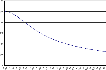
Lets begin by examining the Fourier transform of a decaying exponential:
![]() , where
, where ![]() is the unit step function, 0 for all
is the unit step function, 0 for all ![]() and 1 for
and 1 for ![]() . This captures the general shape of
the
. This captures the general shape of
the
![]() weighting function, shown in Figure 6.
Its Fourier transform is
weighting function, shown in Figure 6.
Its Fourier transform is
![]() .
The transform attenuates,
but does not eliminate, higher frequency elements. If the input signal
oscillates, the output will oscillate as well. As
.
The transform attenuates,
but does not eliminate, higher frequency elements. If the input signal
oscillates, the output will oscillate as well. As ![]() gets smaller
the higher frequencies are attenuated to a greater degree, but this
corresponds to picking a larger value for
gets smaller
the higher frequencies are attenuated to a greater degree, but this
corresponds to picking a larger value for ![]() in
in
![]() and comes at
the expense of greater lag in response to changing processor load.
and comes at
the expense of greater lag in response to changing processor load.
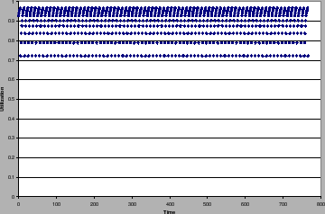
For a specific workload example, we'll use a simple repeating rectangle wave, busy for 9 cycles, and then idle for 1 cycle. This is an idealized version of our MPEG player running roughly at an optimal speed, i.e. just idle enough to indicate that the system isn't saturated. Ideally, a policy should be stable when it has the system running at an optimal speed. This implies that the weighted utilization should remain in a range that would prevent the processor speed from changing. However, as was fore-shadowed by our initial qualitative discussion, this is not the case. A rectangular wave has many high frequency components, and these result in a processor utilization as shown in Figure 7. This figure shows the oscillation for this example, and shows that oscillation occurs over a surprisingly wide range of the processor utilization. As discussed earlier, our experimental results with the MPEG player on the Itsy also exhibit this oscillation because that application exhibits the same step-function resource demands exhibited by our example.
We also simulated interval-based averaging policies that used a pure average rather than an exponentially decaying weighting function, but our simulations indicated that that policy would perform no better than the weighted averaging policy. Simple averaging suffers from the same problems experienced by the weighted averaging if you do not average the appropriate period.