
4th USENIX Symposium on Networked Systems Design & Implementation
Pp. 101–114 of the Proceedings
S4: Small State and Small
Stretch Routing Protocol for
Large Wireless Sensor Networks
Yun Mao  Feng Wang 
Lili Qiu Simon S. Lam
Jonathan M. Smith
The University of Texas at Austin University
of Pennsylvania
Abstract:
Routing protocols for wireless sensor networks must address the
challenges of reliable packet delivery at increasingly large scale and
highly constrained node resources. Attempts to limit node state can
result in undesirable worst-case routing performance, as measured by
stretch, which is the ratio of the hop count of the selected path to that of
the optimal path.
We present a new routing protocol, Small State and Small Stretch
(S4),which jointly minimizes the state and stretch. S4 uses a
combination of beacon distance-vector based global routing state and
scoped distance-vector based local routing state to achieve a
worst-case stretch of 3 using
 routing state per node in
an N-node network. Its average routing stretch is close to 1. S4
further incorporates local failure recovery to achieve resilience to
dynamic topology changes. We use multiple
simulation environments to assess performance claims at scale, and use
experiments in a 42-node wireless sensor network testbed to evaluate
performance under realistic RF and failure dynamics. The results show
that S4 achieves scalability, efficiency, and resilience in a wide range of
scenarios. routing state per node in
an N-node network. Its average routing stretch is close to 1. S4
further incorporates local failure recovery to achieve resilience to
dynamic topology changes. We use multiple
simulation environments to assess performance claims at scale, and use
experiments in a 42-node wireless sensor network testbed to evaluate
performance under realistic RF and failure dynamics. The results show
that S4 achieves scalability, efficiency, and resilience in a wide range of
scenarios.
1 Introduction
Routing finds paths in a network along which to send data. It is one
of the basic network functionalities. The effectiveness of routing
protocols directly affects network scalability, efficiency, and
reliability. With continuing growth of wireless network sizes, it is
increasingly important to develop routing protocols that
simultaneously achieve the following design goals.
- Small routing state: Using small amounts of routing
state is essential to achieving network scalability. Many wireless
devices are resource constrained. For example, mica2 sensor motes
have only 4KB RAM. Limiting routing state is necessary for such
devices to form large networks. Moreover, limiting routing state
also helps to reduce control traffic used in route setup and
maintenance, since the
amount of routing state and control traffic is often correlated.
- Small routing stretch: Routing stretch is defined as the ratio between the cost of
selected route and the cost of optimal route. Small routing stretch
means that the selected route is efficient compared to the optimal
route. It
is a key quantitative measure of route quality, and
affects global resource consumption, delay, and reliability.
- Resilience: Wireless networks often experience frequent topology
changes arising from battery outage, node failures, and
environmental changes. Routing protocols should find efficient routes
even in the presence of such changes.
Existing routing protocols either achieve small worst-case routing stretches
with large routing state (e.g., shortest path routing) or achieve
small routing state at the cost of large worst-case routing stretches
(e.g., geographic routing and hierarchical routing). In this paper, we
present the design and implementation of Small State and Small Stretch
(S4), a new addition to the routing protocol design space. S4
achieves a desirable balance among these characteristics, and is well suited to the
wireless sensor network setting.
We make the following contributions.
- S4 is the first routing protocol that achieves
a worst-case routing stretch of 3 in large wireless networks.
Its average routing stretch is close to 1.
- S4's distance guided local failure recovery scheme significantly
enhances network resilience, and is portable to other settings.
- S4's scalability, effectiveness of resource use, and resilience are
validated using multiple simulation environments and a 42-node sensor
network testbed.
The rest of the paper is organized as follows. In
Section 2, we discuss the limitations of previous
work. We present the S4 routing protocol in
Section 3.
We evaluate its performance using high-level
simulation in Section 4,
to study the performance under ideal wireless environment
with no wireless medium losses or collisions.
In Section 5, we
present evaluation results using TOSSIM, a packet-level simulator that
models wireless medium and collisions, to study the performance
in more realistic large-scale wireless networks. In
Section 6 we describe testbed evaluation. We
conclude in Section 7.
2 Related Work
Routing is a well-studied problem, but wireless
sensor networks have introduced new challenges.
Shortest path routing protocols (e.g., DSR [10],
AODV [22], DSDV [21]) can find good routes,
but are limited in scale by both
control traffic and the amount of state required at each node.
Consequently, routing in large-scale wireless networks has
focused on minimizing storage and exchange of routing state, and
can be divided
into geographic routing and
hierarchical routing approaches.
In geographic routing, each node is assigned a coordinate
reflecting its position in the network. Upon receiving a packet, a node
selects a next hop closer to the destination in the
coordinate space. Some geographic routing protocols use geographic
locations as node coordinates, while others use virtual coordinates
based on network proximity. As connectivity in the coordinate
spaces is not complete, these schemes must address getting ``stuck'' in
a local minimum, where no neighbor is closer to the destination
than the current node.
Some proposals such as GFG [1],
GPSR [11], GOAFR+ [14],
GPVFR [17] and variants use face traversal schemes
that route packets on a planar graph derived from the original
connectivity graph. Their delivery guarantees [5]
depend on the assumption that the planarization algorithms (e.g.
GG [6] and RNG [27]) can successfully planarize any
network graph. These planarization algorithms typically assume a unit
disk or quasi-unit disk model. However, these models can be
inadequate for
real wireless environments due to obstacles and
multi-path fading. Kim, et.
al [13] have shown that model failures in
real radio environments can cause routing pathologies and persistent routing
failures. CLDP [12] addresses
the imperfect
RF propagation problem using a right-hand probing rule
to detect link-crossings and
remove them to re-planarize the graph.
GDSTR [16] provides delivery guarantee without requiring
planarization
by avoiding routing across the face of planar graphs and
instead routing packets
through a spanning tree.
The geographic coordinate-based routing schemes have at least three
difficulties for wireless sensor networks.
First, accurate geolocation either requires careful static setting or access
to GPS, with consequences for cost and need for line-of-sight to satellites.
Second,
geographic distances may lack predictive value for network
performance (e.g., loss rate). This may result in paths with poor performance.
Third, even with GPS and ideal
radios, the best routing stretch
for geographic routing is  in GOAFR+ [14] and ARF [15], where in GOAFR+ [14] and ARF [15], where  is the length of the optimal path,
and example topologies exist where this bound
is tight
[15].
is the length of the optimal path,
and example topologies exist where this bound
is tight
[15].
Virtual coordinates reflecting underlying network connectivity
address the first two difficulties, but still face the challenge
of ``dead ends'', for which a recovery scheme is required.
In addition, the overhead of computing and storing virtual
coordinates is not negligible.
For example,
NoGeo [24]
uses
perimeter nodes to flood
the  -node network so that every node can learn its distances to all
the perimeter nodes. Each node determines its virtual coordinate based
on the distances to the perimeter nodes. However, perimeter nodes need
to store -node network so that every node can learn its distances to all
the perimeter nodes. Each node determines its virtual coordinate based
on the distances to the perimeter nodes. However, perimeter nodes need
to store
 pair-wise distance amongst them, which is not scalable in
large wireless networks with limited memory space per node.
GEM [20] achieves greater scalability
by using triangulation from a root node and two
other reference nodes. However, the routing stretch is larger
than that typical of geographic routing algorithms,
and there is the additional cost of recomputing
routing labels resulting from network failures.
Fonseca, et al. [4]
have proposed Beacon Vector Routing (BVR) which selects a few
beacon nodes, and uses flooding to construct spanning trees from the
beacons to all other nodes. A node's coordinate is a vector of
distances from the node to all beacons, and each node maintains the
coordinates of its neighbors. BVR defines a distance metric over
these beacon vectors, and a node routes packets to the one that minimizes the
distance. When greedy routing stalls, it
forwards the packet towards the beacon closest to the destination. If
the beacon still fails to make greedy progress, scoped flooding is used.
None of the virtual coordinate-based routing algorithms provide worst-case
routing stretch guarantees. pair-wise distance amongst them, which is not scalable in
large wireless networks with limited memory space per node.
GEM [20] achieves greater scalability
by using triangulation from a root node and two
other reference nodes. However, the routing stretch is larger
than that typical of geographic routing algorithms,
and there is the additional cost of recomputing
routing labels resulting from network failures.
Fonseca, et al. [4]
have proposed Beacon Vector Routing (BVR) which selects a few
beacon nodes, and uses flooding to construct spanning trees from the
beacons to all other nodes. A node's coordinate is a vector of
distances from the node to all beacons, and each node maintains the
coordinates of its neighbors. BVR defines a distance metric over
these beacon vectors, and a node routes packets to the one that minimizes the
distance. When greedy routing stalls, it
forwards the packet towards the beacon closest to the destination. If
the beacon still fails to make greedy progress, scoped flooding is used.
None of the virtual coordinate-based routing algorithms provide worst-case
routing stretch guarantees.
Hierarchical routing is an alternative approach to achieving
scalability. Example protocols in this category include landmark
routing [28], LANMAR [7], ZRP [8] and
Safari [23]. Hierarchical routing protocols provide no
guarantee on the routing stretch due to boundary effects: two nodes
that are physically close may belong to different clusters or zones, and hence
the route between them has to go through cluster heads, which can be
arbitrarily longer than their shortest path.
Caesar et al. develop VRR [2], a
scheme for layer-3 any-to-any routing based on
distributed hash tables.
To route to its successors on the virtual ring, a
node sets up and maintains forwarding entries to its successors and
predecessors along multi-hop physical paths. As a result, a node has
both routing table entries towards its neighbors in the ring and also
entries for the nodes on the paths in between. VRR greedily forwards a
packet toward the node in the routing table with the closest ID to the
destination ID. The routing state per node is roughly
. Unlike S4, VRR does not provide worst-case routing stretch
guarantee.
Theoretical work [3,26] on achieving scalable and
efficient routing has developed compact routing algorithms that
provide a worst-case routing stretch of 3 while using at most
 state in an -node network. This worst-case
routing stretch is provably optimal when each node uses less than
linear routing state [3,26].
While compact routing seems to be a promising direction for
large-scale networks, it cannot be directly translated into a routing protocol in a
distributed network. In particular, the proposed algorithms do not
specify how each node should build and maintain routing state for
local clusters and for beacon nodes. Moreover, the algorithm
in [26] requires choosing beacon nodes offline,
considers only initial route construction, and cannot cope
with topology changes, which precludes
realization in our network setting.
The implications of
compact routing for average routing stretch
also remain unclear. state in an -node network. This worst-case
routing stretch is provably optimal when each node uses less than
linear routing state [3,26].
While compact routing seems to be a promising direction for
large-scale networks, it cannot be directly translated into a routing protocol in a
distributed network. In particular, the proposed algorithms do not
specify how each node should build and maintain routing state for
local clusters and for beacon nodes. Moreover, the algorithm
in [26] requires choosing beacon nodes offline,
considers only initial route construction, and cannot cope
with topology changes, which precludes
realization in our network setting.
The implications of
compact routing for average routing stretch
also remain unclear.
3 S4 Routing Protocol
S4 uses the theoretical ideas of the compact routing
algorithm [26] as a
basis, refined by the addition of new techniques needed
to obtain a
practical routing protocol for large-scale wireless networks.
We first describe
the basic routing algorithm and note challenges for routing
protocol design, and then present the S4 routing protocol. Throughout this
paper, our metric for
the cost of a route is the number of links traversed
(i.e., hop count).
3.1 Basic Routing Algorithm
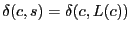
In S4, a random set of nodes,  , are chosen as beacons. For a node , are chosen as beacons. For a node
 , let , let  denote the beacon closest to node , and let denote the beacon closest to node , and let
 denote the shortest path distance from denote the shortest path distance from  to . Each
node constructs the following local cluster, denoted as to . Each
node constructs the following local cluster, denoted as  .
where .
where  is the set of all nodes in the network.
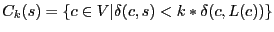
A local cluster of node consists of all nodes whose distances to
are within is the set of all nodes in the network.
A local cluster of node consists of all nodes whose distances to
are within  times their distances to their closest
beacons. Each node
then maintains a routing table for all beacon nodes and nodes in its
own cluster . times their distances to their closest
beacons. Each node
then maintains a routing table for all beacon nodes and nodes in its
own cluster .
Figure 1:
S4 routing examples. Every node within the circle of has
in its local cluster. The route
 is
the shortest path; the route is
the shortest path; the route
 takes a
shortcut at before reaching ; the route takes a
shortcut at before reaching ; the route
 is
through is
through  without shortcut. without shortcut.
|
As shown in Figure 1, when routing from node to
node , if
 , we can directly use the shortest path to
route from to . Otherwise, first takes the shortest path towards
, and then use the shortest path to route
towards . In the second case, the route does not
have to always reach before routing to . Whenever data
reaches a node whose cluster contains , can directly route
to using the shortest path from to . According to the
triangle inequality, the ``shortcut'' strictly improves routing
stretch. We give the following theorem as an extension
to the proof in [3,26], in which a special case , we can directly use the shortest path to
route from to . Otherwise, first takes the shortest path towards
, and then use the shortest path to route
towards . In the second case, the route does not
have to always reach before routing to . Whenever data
reaches a node whose cluster contains , can directly route
to using the shortest path from to . According to the
triangle inequality, the ``shortcut'' strictly improves routing
stretch. We give the following theorem as an extension
to the proof in [3,26], in which a special case  is proved. Refer to our technical report [19] for the proof.
Theorem 1
Let
 , where , where  . If each node maintains next-hop for the shortest path to
every beacon and every node in , the worst-case routing
stretch is . If each node maintains next-hop for the shortest path to
every beacon and every node in , the worst-case routing
stretch is
 . .
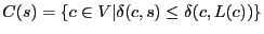
As a special case, when , a local cluster of node consists of
all nodes whose distances to are closer than their distances to
their closest beacons. This special case is called compact
routing [3,26]. It is particularly interesting, since it has low worst-case
storage cost of
 and provides a worst-case routing stretch of 3.
In the remaining paper we consider , since it gives small
routing state. and provides a worst-case routing stretch of 3.
In the remaining paper we consider , since it gives small
routing state.
Practical concerns dictate three changes to
the TZ compact routing
scheme [26] to achieve S4. First, the boundary conditions of
the cluster definitions are slightly different. In S4,
 , but in the TZ scheme, , but in the TZ scheme,
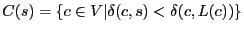 . That is, node
is in the cluster of in S4 but not in the TZ scheme, if . That is, node
is in the cluster of in S4 but not in the TZ scheme, if
 . This change does not affect the worst-case routing
stretch, and reduces average-case routing stretch at the cost of increasing
routing state. . This change does not affect the worst-case routing
stretch, and reduces average-case routing stretch at the cost of increasing
routing state.
Second, to route towards node , only should be carried
in the packet header as the location information in S4. In comparison,
the TZ scheme requires a
 for each
packet, where for each
packet, where
 is the next hop at towards .
Only with the label carried in the packet header, a beacon node can
forward a packet towards using next hop
. It is
necessary in the TZ scheme because the beacon nodes do not store
routing state. However, in S4, as a result of the boundary condition
change, each beacon node stores routing state to all the nodes
that have as its closest beacon node. Given that the total storage cost
of the additional field
in the labels is the same as
the total number of routing entries at beacon nodes in S4 (i.e., both
are N), we favor storing
routing state at beacon nodes since it reduces packet header length
and the frequency of updating labels. The frequency of label updates
is reduced because labels are updated only when changes but not
when
changes. is the next hop at towards .
Only with the label carried in the packet header, a beacon node can
forward a packet towards using next hop
. It is
necessary in the TZ scheme because the beacon nodes do not store
routing state. However, in S4, as a result of the boundary condition
change, each beacon node stores routing state to all the nodes
that have as its closest beacon node. Given that the total storage cost
of the additional field
in the labels is the same as
the total number of routing entries at beacon nodes in S4 (i.e., both
are N), we favor storing
routing state at beacon nodes since it reduces packet header length
and the frequency of updating labels. The frequency of label updates
is reduced because labels are updated only when changes but not
when
changes.
Finally, the TZ scheme proposes a centralized beacon node selection
algorithm to meet expected worst case storage bound
in an -node network. Since practicality is our main design
goal, in S4 we randomly select beacon nodes in a distributed fashion.
It is proved that
when
nodes are randomly selected as beacon nodes, the
average storage cost on each node is still
[25]. As our evaluation results show, the
storage cost is still low even for the worst cases. Note that the
worst-case routing stretch of 3 still holds under random beacon node
selection.
3.2 Design Challenges
Designing a routing protocol to realize the algorithm proposed in
Section 3.1 poses the following challenges:
First, how to construct and maintain routing state for a local
cluster? Frequent topology changes in wireless networks make it
necessary to support incremental routing updates. Unlike traditional
hierarchical routing, each node has its own cluster in compact
routing. Therefore naive routing maintenance could incur significant
overhead.
Second, how to construct and maintain routing state for beacon
nodes? Knowledge of next-hops and shortest path distances to beacon
nodes is important to the performance of S4. When beacon packets are
lost, the routing state could be inaccurate, which could
substantially degrade the performance.
Third, how to provide resilience against node/link failures and
environmental changes? Maintaining up-to-date routing state could
be expensive especially in a large network. Moreover routing changes
take time to propagate. During the transient period (e.g., the
period from the time when failure occurs to the time when the
routing tables at all nodes are updated to account for the failure),
many packets could be lost without a failure recovery scheme.
To address the above challenges, S4 consists of the following three major
components: (i) scoped distance vector for building and maintaining
routing state to nodes within a cluster, (ii) resilient beacon
distance vector for efficient routing towards beacon nodes and
facilitating inter-cluster routing, and (iii) distance guided local failure
recovery for providing high quality routes even under dynamic
topology changes. Below we will describe these three components in turn.
3.3 Intra-Cluster Routing: Scoped Distance Vector (SDV)
In S4, node uses the shortest paths to route towards nodes in the
cluster of . Unlike the traditional hierarchical routing, in S4
each node has its own cluster, which consists of nodes close to
node . This clustering is essential for providing a routing stretch
guarantee, since it avoids boundary effects. In comparison,
hierarchical routing cannot provide routing stretch guarantee due to
boundary effects, where two nearby nodes belong to different clusters
and the hierarchical route between them could be much longer than
their direct shortest path.
A natural approach to building a local routing table is to use scoped
flooding. That is, each node floods the network up to
 hops away from , where
is the distance between and its
closest beacon . Scoped flooding works fine when the network is
initialized, or when there are new nodes joining the network. But
it is costly to send frequent scoped floodings to reflect constant topology changes,
which often arises in wireless networks due to battery outage, node
failures, and environmental changes. hops away from , where
is the distance between and its
closest beacon . Scoped flooding works fine when the network is
initialized, or when there are new nodes joining the network. But
it is costly to send frequent scoped floodings to reflect constant topology changes,
which often arises in wireless networks due to battery outage, node
failures, and environmental changes.
Scoped distance vector: To provide cheap incremental routing
updates, we propose using scoped distance vector (SDV) for
constructing routing tables for local clusters. SDV is attractive
because it is fully distributed, asynchronous, and supports
incremental routing updates. SDV is more efficient than scoped
flooding especially under small changes in a network topology, because
a node in SDV propagates
routing update only when its distance vector changes while in scoped
flooding a node propagates a flooded packet regardless of
whether its distance and next hop to a destination have changed.
In S4, each node stores a distance vector for each destination
in its cluster as the
following tuple:
where and
 are both node IDs, are both node IDs,  is the
latest sequence number for destination , and is the
latest sequence number for destination , and  is the distance between and 's closest beacon, and
  is
whether the distance vector has been updated since the last routing update. is
whether the distance vector has been updated since the last routing update.
A node exchanges its distance vectors with its neighbors either
synchronously or asynchronously. Node initializes
 for only for only
 , and , and  otherwise. Upon receiving a distance vector, a
node uses the newly received distance vectors to update its
routing state. Node further propagates the update for only when
its current distance from is below
otherwise. Upon receiving a distance vector, a
node uses the newly received distance vectors to update its
routing state. Node further propagates the update for only when
its current distance from is below  and its distance
vector to has changed. and its distance
vector to has changed.
Benefits of SDV: SDV supports incremental routing updates. This
allows a wireless network to dynamically adapt to routing changes.
Moreover, unlike traditional distance vector protocols,
SDV does not suffer from the count-to-infinity
problem,1because the scope is typically small (e.g., We evaluate a 1000-node
network with 32
beacons, and its average scope is 3.35 and maximum scope is 13. This
implies routing loops can be detected within 13 hops).
To support routing across clusters, each node is required to know its
distances to all beacons. This can be achieved by constructing
a spanning tree rooted from each beacon nodes to every other node in
the network. Flooding beacon packets reliably is important to the
routing performance, because loss of beacon packets may introduce
errors in estimating the closest beacon and its distance, and degrade
the performance of S4. We develop a simple approach to enhance resilience of beacon packets.
Routing state construction and maintenance: To construct
routing state for beacon nodes, every beacon periodically broadcasts
beacon packets, which are flooded throughout the network. Every node
then keeps track of the shortest hop count and next-hop towards each
beacon.
Since beacon packets are broadcast and typical MAC protocols (e.g.,
CC1000 used in sensor motes) do not provide reliability for broadcast packets, it is
essential to enhance the resilience of beacon packets at the network
layer. Our idea is to have a sender retransmit the broadcast packet
 until until  neighbors have forwarded or until
the maximum retry count neighbors have forwarded or until
the maximum retry count
 is reached. and
provide a tradeoff between overhead and
reliability. In our evaluation, we use is reached. and
provide a tradeoff between overhead and
reliability. In our evaluation, we use
 , ,  for beacon nodes, and for beacon nodes, and
 for non-beacon nodes. for a beacon node is used because
all neighbors of the beacon nodes should forward the beacon
packet. In comparison, for a non-beacon node , only a subset of 's
neighbors are farther away from the beacon than and need to
forward the beacon packet received from . Therefore we use a smaller for non-beacon nodes. for non-beacon nodes. for a beacon node is used because
all neighbors of the beacon nodes should forward the beacon
packet. In comparison, for a non-beacon node , only a subset of 's
neighbors are farther away from the beacon than and need to
forward the beacon packet received from . Therefore we use a smaller for non-beacon nodes.
3.5 Distance Guided Local Failure Recovery (DLF)
Wireless networks are subject to bursty packet losses and frequent
topology changes. To provide high routing success rate and low
routing stretch even in the presence of frequent topology changes and
node/link failures, we develop a simple and effective local failure
recovery based on distance vectors.
Overview: A node retransmits a packet when it does not
receive an ACK within a retransmission timeout. When  retransmissions fail, broadcasts a failure recovery request,
which contains (i) the next hop used, (ii) whether destination is included
in 's local
cluster, and (iii) the distance to if
's cluster includes , or the distance to 's beacon
otherwise. Upon hearing the failure requests, 's neighbors attempt
to recover the packet locally. Our goal is to select the neighbor that
is the closest to the destination as 's new next-hop; meanwhile the
selection process should be cheap and easily distributed.
retransmissions fail, broadcasts a failure recovery request,
which contains (i) the next hop used, (ii) whether destination is included
in 's local
cluster, and (iii) the distance to if
's cluster includes , or the distance to 's beacon
otherwise. Upon hearing the failure requests, 's neighbors attempt
to recover the packet locally. Our goal is to select the neighbor that
is the closest to the destination as 's new next-hop; meanwhile the
selection process should be cheap and easily distributed.
S4 uses distance guided local failure recovery to prioritize
neighbors' responses based on their scoped distance vectors. Each
node uses its priority to determine the time it needs to wait before
sending failure recovery response. We further exploit broadcast
nature of wireless medium to avoid implosion of recovery responses.
Distance guided local failure recovery: Our goal is to
prioritize neighbors based on their distances to the destination so that
the nodes closest to the destination can take over the forwarding. The
problem is non-trivial, because the distance to the destination is not
always available. When the destination is outside the local cluster,
a neighbor only knows the distance to the destination's closest beacon, but not
the distance from that beacon to the destination.
To address the issues, each node computes its priority using the
algorithm in Figure 2. It involves two main
scenarios. In the first scenario, 's local cluster contains the
destination . This information is available in 's failure recovery
request. Then 's neighbor is assigned one of the four priorities
using the following rules. The neighbors that have
in their clusters are assigned the top 3 priorities,
since they can directly route towards destination using the shortest
path. In this case, each neighbor knows its distance to the
destination, and assigns itself a priority based on the difference
between
 and
. Neighbors
whose local clusters do not contain the destination are assigned the
fourth priority, which is the lowest. and
. Neighbors
whose local clusters do not contain the destination are assigned the
fourth priority, which is the lowest.
In the second case, when 's cluster does not contain the destination
, only the neighbors that have in their clusters
are assigned the highest priority, since they can directly route
towards the destination. The other nodes are assigned priorities by
comparing their distances to the beacon with
 . .
A sender selects the neighbor from which it receives the response
first as the new next-hop. By assigning each neighbor  with a timer with a timer
 , a higher priority node sends the response
earlier and is thus favored as the new next-hop node. To avoid
collisions, we add a small random timer , a higher priority node sends the response
earlier and is thus favored as the new next-hop node. To avoid
collisions, we add a small random timer  to the priority-based
timer so that different nodes are likely to respond at different times
even when assigned the same priority. To avoid response implosion,
upon hearing a failure response to from someone else, the current node cancels its own
pending recovery response if any. Our evaluation uses to the priority-based
timer so that different nodes are likely to respond at different times
even when assigned the same priority. To avoid response implosion,
upon hearing a failure response to from someone else, the current node cancels its own
pending recovery response if any. Our evaluation uses  , and , and
 ranges from 0 to 49ms. ranges from 0 to 49ms.
Figure 2:
Computing priority using scoped distance vectors and beacon
distance vectors
|
Node failures vs. link failures: The above scheme works well
for link failures. When a node fails, all the links to and from the
failed nodes are down. Therefore we need to avoid using nodes that use
the failed nodes as next hop. This can be done by letting the sender
specify the failed node. Only the nodes that use different next hop
from the failed node will attempt to recover. In practice, it is
difficult to distinguish between a link failure and a node
failure. Always assuming a node failure may unnecessarily prune out good next-hops.
So we first optimistically assume that the next hop does not fail, only
the link is down. Therefore we allow nodes with
the same next hop to recover the packet. When the number
of failed attempts pass a threshold, we prevent the nodes from using the same next hop
to recover the packet.
3.6 Other Design Issues
Location directory: So far we assume that the source knows
which beacon node is closest to the destination. In practice, such
information may not be directly available. In such situation, the
source can apply the location directory scheme described in
BVR [4] to lookup such information. More specifically, beacon
nodes are responsible for storing the mapping between non-beacon nodes
and their closest beacons. The closest beacon information for node
is stored at H(i), where H is a consistent hash function that maps
nodeid to beaconid. The source contacts the beacon node whose ID
is H(dest) to obtain the closest beacon to dest. The storage cost
of location directory is much smaller in S4 than that in BVR (as shown
in Section 4), because the source in S4 only needs to know
the closest beacon to its destination while the source in BVR needs to
know the distance between its destination and all beacon nodes.
Moreover, in S4 when destination is in 's cluster, no location
lookup is required since knows the shortest path to , whereas
BVR as well as other geographic routing schemes always require
location lookup on a new destination. Such property is especially
beneficial when traffic exhibits locality (i.e., nodes close to each
other are more likely to communicate).
Beacon maintenance: When a beacon fails, S4 applies
distance guided local failure recovery to temporarily route around the
failure. If the failure persists, we can apply the beacon maintenance
protocol proposed in [4] to select a new beacon. Beacon
maintenance is not the focus of this paper. Instead,
we focus on the routing performance during the
transient period after failures occur.
Link quality: Link quality significantly affects routing
performance. We define link quality as the delivery rate of packet on
the link in a given direction. In S4, each node continuously monitors
its links to/from its neighbors. We adopt a passive link estimator
layer developed in [29,4] for estimating link quality. When
a node receives a beacon packet or SDV update, it first checks if both the forward and reverse link qualities of the sender are above a
threshold (30% is used in our current implementation). Only those
updates from a sender with good link quality in both directions will be accepted.
4 Simulation
In this section, we evaluate the efficiency and scalability of S4 by
simulation. We compare S4 with BVR [4], because BVR is one of
the latest scalable routing protocols and also among the few that have
been implemented in real sensor networks. We use BVR with scoped
flooding since it provides delivery guarantee and offers a fair
baseline comparison. We use three evaluation methodologies: (i) MATLAB
simulation based on the unit disk graph radio model (presented in this
section), (ii) TOSSIM simulation, a packet-level simulator with more
detailed wireless model (presented in Section 5), and
(iii) testbed evaluation (presented in
Section 6). Our MATLAB simulation results can be
directly compared with many previous work on geographic routing, in
which the unit disk model is used. TOSSIM simulations allow us to
study the performance in more realistic large-scale wireless
networks. Having both levels of simulations also reveals how
underlying wireless models may affect the routing performance. For
BVR, we validate our matlab implementation of BVR by comparing with
the original BVR simulation code, and we directly use the original BVR
implementation in TinyOS for TOSSIM evaluation.
To study the protocols in an ideal wireless environment, N nodes are
randomly placed in a square rectangle region of size A^2 in the
simulator. The packet delivery rates among nodes are derived from the
unit disk graph model. That is, each node has a fixed communication
range R. A node can communicate with all the nodes inside R, but
cannot communicate with any node outside R. It is also assumed that
there is no packet loss, collision, or network congestion. In the
following description, we let N denote the number of nodes, K
denote the number of beacon nodes, R denote communication range, and
A^2 denote the size of the area.
We use the following performance metrics to quantify the efficiency
and robustness of S4:
- Routing stretch: the ratio of the route length
using the selected routing protocol to that
using the optimal shortest path routing protocol.
- Transmission stretch: the ratio of the total number of
packets transmitted using the selected routing protocol to that
using the optimal shortest path routing protocol.
- Routing state: the amount of state required to maintain at each node.
- Control traffic: the amount of traffic transmitted for setting up the
routing state and location directory.
Unless specified otherwise, our default simulation scenario uses a
3200-node network with nodes uniformly distributed in an area of
 square units. The communication range is 1 unit. On
average each node has 15.4 immediate neighbors. Beacon nodes are randomly
selected. In BVR, all or a subset of beacon nodes serve as routing
beacons; a node's coordinate is defined as its distances to the routing
beacons.
The number of
routing beacons square units. The communication range is 1 unit. On
average each node has 15.4 immediate neighbors. Beacon nodes are randomly
selected. In BVR, all or a subset of beacon nodes serve as routing
beacons; a node's coordinate is defined as its distances to the routing
beacons.
The number of
routing beacons  is fixed to 10 for all simulations,
because it is reported to offer a good balance between
routing performance and overhead [4].
For each configuration, we conduct 10 random runs and report
the aggregate statistics. is fixed to 10 for all simulations,
because it is reported to offer a good balance between
routing performance and overhead [4].
For each configuration, we conduct 10 random runs and report
the aggregate statistics.
Figure 3:
S4 has routing and transmission stretches close to 1, which
is consistently smaller than those of BVR algorithms across all
numbers of beacons.
|
|
Routing and transmission stretches: First we compare the routing and transmission stretches of S4 and two
variants of BVR by varying the number of beacons K. BVR 1-hop refers to the default BVR algorithm. BVR
2-hop is an on-demand 2-hop neighbor acquisition. In this approach, when a node cannot use
greedy forwarding to make progress, it fetches its 1-hop neighbors'
neighbors to its routing table. BVR 2-hop reduces the routing failure
rate of BVR 1-hop at the cost of higher routing state and control
traffic.
Figure 3(a) compares the routing stretches under
S4, BVR 1-hop, and BVR 2-hop. The stretches are computed based on
32,000 routes between randomly selected pairs of nodes. We observe that S4 has the lowest average
routing stretch. A closer examination of the simulation results
shows that the worst stretches in S4 are bounded by 3.
This is consistent with the worst-case guarantee provided by
S4. In comparison, the average routing stretches in BVR 1-hop and 2-hop are
substantially higher especially for small K. Moreover their
worst-case routing stretches are even higher
(e.g., the worst routing stretch of BVR 1-hop in the simulation is 6 for K=56,
and much larger for smaller K).
Figure 3(b) compares transmission stretch among
the three routing protocols. The average transmission stretches of S4
are consistently below 1.1 under all values of K. However,
both BVR 1-hop and BVR 2-hop have much higher stretches when K is
small. To achieve comparable transmission stretches to
S4 (though still higher), the least numbers of beacons required is 56 for BVR 1-hop and 30
for BVR 2-hop. Such high transmission stretch in BVR is due
to its scoped flooding, which is necessary for its guaranteed delivery.
Figure 4:
Routing state comparison: When
 , the routing state in
S4 is half of routing state in BVR. , the routing state in
S4 is half of routing state in BVR.
![\includegraphics[width=1.55in]{fig/state.eps}](fig4.png)
|
Routing state: Figure 4 compares routing state
per node under the three routing protocols. The routing state in S4
include route entries for beacon nodes and for nodes within
local clusters, whereas the routing state in BVR are determined by
the number of neighbors and the length of their beacon vectors K.
2 We make the following observations. First, in BVR
the average routing table size proportionally increases with
the number of beacons, while the number of entries remains close to
the number of neighbors. In comparison, the routing state in S4 first
decreases and then slightly increases with the number of beacon
nodes. The routing state in S4 reaches minimum for
 since it gives a good balance between global routing state (for
beacon nodes) and local routing state (for nodes in the
clusters). These trends also hold for maximum routing state in BVR
and S4. Second, recall that to achieve a relatively small
transmission stretch, 56 beacon nodes are required in BVR. In this
case, the average and maximum routing state in BVR is twice or more
than those of S4. Third, BVR
2-hop has significantly higher upper bound of routing state than BVR 1-hop due to
the requirement of holding 2-hop neighbor information.
since it gives a good balance between global routing state (for
beacon nodes) and local routing state (for nodes in the
clusters). These trends also hold for maximum routing state in BVR
and S4. Second, recall that to achieve a relatively small
transmission stretch, 56 beacon nodes are required in BVR. In this
case, the average and maximum routing state in BVR is twice or more
than those of S4. Third, BVR
2-hop has significantly higher upper bound of routing state than BVR 1-hop due to
the requirement of holding 2-hop neighbor information.
Figure 5:
Initial control traffic to set up routing state: the
errorbars show minimum, mean, and maximum traffic across all
nodes. The control traffic of S4 decreases gracefully as the number of
beacons increases. When
, the overhead of S4 is 65%
higher than that of BVR 1-hop, but much less than BVR 2-hop.
![\includegraphics[width=1.55in]{fig/traffic.eps}](fig5.png)
|
Control traffic: Figure 5 shows
initial control traffic for setting up routing state. The bandwidth overhead of
BVR 1-hop increases linearly with the number of beacons, because the
main overhead is the beacon flooding messages. In BVR 2-hop, other
than beacon flooding, the control traffic also includes the overhead
of fetching 2-hop neighbor coordinates for the required nodes. We can
see the overhead of on-demand 2-hop neighbor acquisition is
significant, which is a big disadvantage of BVR 2-hop even though its
routing stretch is lower than BVR 1-hop. In S4, control traffic includes beacon flooding and SDV. As K
increases, the size of the local cluster of each node decreases, so
the number of scoped DV packets is reduced. When K=56, the overhead
of S4 is 65% higher than that of BVR 1-hop. However since SDV can be
updated incrementally after the initial setup, its amortized overhead
over the long run is reduced. In terms of the number of packets, S4 is
less than twice of the BVR 1-hop when
K >= sqrt(N). Note that the
number of packets in S4 can be reduced by grouping SDV packets. On the
other hand, BVR demands large packet size when the number of beacons is
large, and large packets could be forced to split in order to achieve
high delivery rates under unreliable links.
Figure 6:
Control traffic overhead of updating routing state due to
topology changes
![\includegraphics[width=1.55in]{fig/dv_only.eps}](fig6.png)
|
To evaluate the overhead of incremental SDV in
S4, we randomly select non-beacon nodes to fail between two
consecutive routing updates to create topology changes. There are two
ways of updating the routing state after the initial round: either
incrementally update based on the current routing state (incremental
DV), or builds new routing tables starting from scratch (regular DV).
As shown in Figure 6, when the number of node failures
is small (e.g., within 5%), incremental routing updates incur lower
overhead. Since the typical number of node failures between
consecutive routing updates is likely to be low, incremental routing
updates are useful in real networks.
Figure 7:
Control traffic overhead comparison
|
|
The control traffic to set up the routing table is not the only
overhead. The source should be able to lookup the location information
of the destination. Therefore, each node should store its location to a
directory during the setup phase. We study such directory setup
overhead by using the location directory scheme described
in 3.6:
each node v periodically publishes its location to a
beacon node b_v by using a consistent hashing mechanism.
b_v
then sends a confirmation back to v if the publishing is successful.
We simulate the initial directory setup overhead, in
which every node publishes its location to the distributed
directory. The results are shown in
Figure 7 (a), and they include traffic to
and from beacon nodes for publishing the locations. S4 has the
following three
advantages over the BVR. First, the size of location information in
S4 is significantly smaller than that of BVR, because in BVR a node's
coordinate is proportional to the number of beacons, while in S4 a node's coordinate is its closest beacon ID.
Second, the transmission
stretch of BVR is higher than that of S4. Therefore, it incurs more traffic in
routing a confirmation packet from the beacon node back to the node publishing
its location. Third, it is more
likely that a node changes its coordinates in BVR than it changes
its closest beacon in S4. Therefore, S4 incurs a lower
overhead in setting up and maintaining the location directory.
Figure 7(b) shows the overall traffic overhead incurred
in setting up both routing state and directory. We observe that
compared with both variants of BVR, S4 has smaller overall control
traffic, including traffic in setting up both route and location directory.
Per data packet header overhead:
Aside from the control traffic, routing protocols also have overhead
in the data packet headers. The overhead of S4 includes the closest
beacon ID to the destination and its distance. For BVR, the overhead
mainly depends on the number of routing beacons . The packet header
of BVR includes a -long destination coordinate, which has at least
 bits indicating which
K beacons as the routing beacons for
the destination. For example, a rough estimation suggests that with
K=56 and =10, BVR requires 15-byte packet headers, which is
significant compared to the default packet payload size of 29 bytes in mica2 motes, while S4 only takes 3 bytes in the packet header. bits indicating which
K beacons as the routing beacons for
the destination. For example, a rough estimation suggests that with
K=56 and =10, BVR requires 15-byte packet headers, which is
significant compared to the default packet payload size of 29 bytes in mica2 motes, while S4 only takes 3 bytes in the packet header.
Figure 8:
Transmission stretch comparison between S4 and BVR
in the presence of obstacles.
|
We now study the performance of S4 and BVR in the presence of
obstacles using the same methodology as in [4].
The obstacles are modeled as horizontal or vertical walls,
which completely block wireless signals. (They do not reflect wireless
signals.) We vary the number and length of those randomly placed
obstacles. We find that the median transmission stretches of S4 and BVR
are 1.00 and 1.04, respectively. They are both
insensitive to the obstacles. However, as shown in
Figure 8, the 95th percentile of the
transmission stretches of S4 and BVR are quite different:
S4 has a constant 95th percentile stretch
around 1.2 regardless the existence of obstacles, while the
transmission stretch of BVR increases with the number of the obstacles
and the length of the obstacles. For example, when there are 75
obstacles with length 2.5 times of the transmission range, 12.9% of
the links are blocked by them. As a result, the 95th percentile
transmission stretch of BVR increases up to 7.9 due to the irregular
topology, while the stretch of S4 stays around 1.2. This is because
S4's worst-case routing stretch guarantee is independent of network
topologies.
Our evaluation shows that S4 provides a worst-case
routing stretch of 3 and an average routing stretch around 1.1 - 1.2
in all evaluation scenarios. When
(a favorable
operating point for both S4 and BVR), S4 has significantly smaller routing state
than BVR. While the initial route setup traffic in S4 is higher than that
of BVR,
due to its compact location representation, its total control traffic
including location setup is still comparable to that of
BVR. Furthermore S4 can efficiently adapt to small topology changes using
incremental routing update. Finally, BVR 1-hop is more scalable than
BVR 2-hop due to its lower control traffic and routing state. So in
the following evaluation, we only consider BVR 1-hop as a baseline comparison.
5 TOSSIM Evaluation
We have implemented a prototype of S4 in nesC language
for TinyOS [9].
The implementation can be directly used both in TOSSIM
simulator [18] and on real sensor motes.
In this section, we evaluate the performance of S4 using
extensive TOSSIM packet-level simulations. By taking into
account actual packet transmissions, collisions, and losses,
TOSSIM simulation results are more realistic.
Our evaluation considers a wide range of scenarios by varying the
number of beacon nodes, network sizes, network densities, link loss
rates, and traffic demands. More specifically, we consider two types
of network densities: a high density with an average node degree of
16.6 and a low density with an average node degree of 7.6. We use both
lossless links and lossy links that are generated by LossyBuilder in TOSSIM. Note that even when links are lossless,
packets are still subject to collision losses. In addition, we examine
two types of traffic: a single flow and 5 concurrent flows. The
request rate is one flow per second for single-flow traffic, and
5 flows per second for 5-flow traffic. The simulation lasts for 1000 seconds.
So the total number of routing requests is 1000 for single-flow traffic,
and 5000 for 5-flow traffic.
We compare
S4 with BVR, whose implementation is available from the public CVS
repository of TinyOS.
5.1 Routing Performance
First we compare S4 with BVR in stable networks. To achieve stable
networks, we let each node periodically broadcast RBDV and SDV packets
every 10 seconds. Data traffic is injected into the network only after
route setup is complete. BVR uses scoped flooding after a packet falls
back to the closest beacon to the destination and greedy forwarding still
fails, whereas S4 uses the distance guided failure recovery
scheme to recover failures. To make a fair comparison, in both BVR and S4
beacon nodes periodically broadcast and build spanning trees, and RBDV
is turned off in S4.
5.1.1 Varying the number of beacons
We vary the number of beacon nodes from 16 to 40 while fixing the total number of
nodes to 1000.
Routing success rate: We study 4 configurations: a single flow
with lossless links, a single flow with lossy links,
5 flows with lossless links, and 5 flows with lossy
links. In the interest of space, Figure 9 only shows the
results of the first and last configurations. ``HD'' and ``LD''
curves represent results under high and low network densities,
respectively.
Figure 9:
Compare routing success under different numbers of
beacons, network densities and traffic patterns.
|
|
We make the following observations. First, under lossless links with 1
flow, S4 always achieves 100% success rate. In comparison, BVR
achieves close to 100% success only in high-density networks, but its
success rate reduces to 93% under low network density with 16
beacons. Why BVR does not provide delivery guarantee
even under perfect channel condition? After a packet is stuck
at the fallback beacon, scoped flooding is used, which
could cause packet collisions and reduce packet
delivery rate. Second, under lossy links with 5 flows, packet losses
are common, and the performance of both S4 and BVR degrades. Nevertheless,
S4 still achieves around 95% routing success rate in high-density networks,
while success rate of BVR drops dramatically. The large drop in BVR is
because its scoped flooding uses broadcast packets, which have no
reliability support from MAC layer; in comparison, data packets are
transmitted in unicast under S4, and benefit from link layer
retransmissions. Third, the success rate is lowest under low-density
networks, with lossy links and 5 flows. Even in this case S4 achieves 70% - 80%
success rate, while the success rate of BVR is reduced to below 50%.
Figure 10:
Compare routing stretch under different numbers of
beacons, network densities, and traffic patterns.
|
Routing stretch: Figure 10 compares the average
routing stretch of S4 and BVR.
The average routing stretch is computed only for the packets that have been
successfully delivered.
Although the worst stretch of S4 is 3, its average
stretch is only around 1.1 - 1.2 in all cases. In comparison, BVR has
significantly larger routing stretch: its average routing stretch is
1.2 - 1.4 for 1 flow, and 1.4 - 1.7 for 5
flows. Moreover its worst routing stretch (not shown) is
8.
Transmission Stretch: As
shown in Figure 11(a), the transmission stretch of S4 is
close to its routing stretch, while the transmission stretch of BVR is
much larger than its routing stretch due to its scoped
flooding. Figure 11(b) shows CDF of transmission stretches
under 32 beacon nodes. We observe that the worst-case
transmission stretch in S4 is 3, and most of the packets have
transmission stretch very close to 1.
Figure 11:
Transmission stretch comparison
|
Control traffic overhead: Compared with BVR, S4 introduces extra control
traffic of SDV to construct routing tables for local clusters.
To evaluate this overhead, we count the average control traffic
(in bytes and number of packets)
that each node generates under lossless links and a single flow.
We separate the global beacon traffic
and local SDV traffic. The results are shown in Figure 12.
Note that beacon traffic overhead is the same for both S4 and BVR.
Figure 12:
Control traffic overhead under different numbers of beacons
and network densities
|
We can see that when the number of beacons is small, the SDV traffic
dominates, since the cluster sizes are relatively large in such
case. As the number of beacons increases, the amount of SDV traffic
decreases significantly. In particular, when there are 32 beacons
(sqrt(1000)), the amount of SDV traffic is comparable to the
amount of global beacon traffic. Moreover, if we include control
traffic for setting up location directory, the total control traffic
in S4 would be comparable to that of BVR, as shown in
Figure 7.
Routing state: We compare routing state of S4 and BVR as follows.
For S4, the routing state consists of a beacon routing table and
a local cluster table. For BVR, the routing state consists of a
beacon routing table and a neighbor coordinate table. We first compare
the total amount of routing state in bytes between S4 and BVR.
Figure 13:
Routing state comparison under different numbers of beacons
and network densities with lossy links (single flow)
|
Figure 13(a) shows the average routing state over all nodes.
We make the following observations.
First, network density has little impact
on the routing state of S4, but has large impact on BVR. This is because
in S4 the local cluster sizes are not sensitive to network density, while in BVR
each node stores the coordinates of its neighbors and its routing
state increases with density. Second, the amount of routing
state in BVR increases with the number of beacons. In comparison, S4's routing state
does not necessarily increase with the number of beacons, since
increasing the number of beacons reduces the local cluster size.
Third, when the number of beacons
is 32
or above, the routing state in S4 is less than BVR. Similar
results have been observed in other TOSSIM configurations as well as MATLAB simulation results in Section 4.
Figure 13(b) further shows the number of entries in
beacon routing table, local cluster table and neighbor coordinate
table. The beacon table curves of S4 and BVR overlap, since it is
common for both. Note that although the coordinate tables in BVR have
fewer entries than the cluster tables in S4, the
total size of the coordinate tables are generally larger since each
coordinate table entry is proportional to the number of beacons.
Table 1 shows maximum routing state of S4 and BVR under
high density and low density.
The maximum number of routing entries is
around 4.5 times of 32(the expected average cluster size),
but still an order of magnitude smaller than 1000 (the flat routing
table size) in shortest path routing. This suggests that random beacon
selection does a reasonable job in limiting worst-case storage cost.
Table 1:
Maximum routing state of S4 and BVR
|
|
max S4 state (B) |
max BVR state (B) |
max S4 routing entries |
|
HD |
680 |
960 |
136 |
|
LD |
715 |
920 |
143 |
|
5.1.2 Varying network size
We also evaluate the performance and scalability of S4 when the network size is varied
from 100 to 4000.
For each network size N, we select
nodes
as beacon nodes. In the interest of space, we only present results under
lossless links and a single flow.
Figure 14:
Comparison under different network sizes
|
Figure 14(a) shows the average transmission stretch of
S4 and BVR under different network sizes. The error bars represent 5-
and 95- percentiles. S4 achieves smaller transmission stretches and
smaller variations in the stretches. In BVR, packets experience higher
medium stretch and higher stretch variation due to greedy forwarding
and scoped flooding.
Figure 14(b) shows the average routing state. For both
S4 and BVR, the routing state tends to increase with
O(\sqrt{N}).
This suggests both S4 and BVR are scalable with network sizes.
In particular, even when the network size is 4000, majority of nodes can
store the routing state in a small portion of a 4KB RAM
(the RAM size on Mica2 motes we experimented with).
Moreover, S4 uses less routing state than BVR when the number of
beacon nodes is , because the coordinate table size in BVR
is linear to the number of beacon nodes.
Table 2:
Performance comparison in 100-node networks.
|
|
success rate |
routing stretch |
transmission stretch |
control traffic (B) |
routing state (B) |
|
S4 |
1 |
1.07 |
1.08 |
96 |
158 |
|
BVR |
0.994 |
1.20 |
1.31 |
46 |
232 |
|
To further study the performance of S4 in smaller networks, we compare
S4 and BVR in networks of 100 nodes. Due to space limitation, we only
include the results for the case of single flow traffic with lossless
links. Table 2 shows that in 100-node networks S4
outperforms BVR in terms of routing success rate, routing stretch,
transmission stretch, and routing state. S4 incurs more control
overhead of BVR due to the extra SDV traffic, though its overall
control traffic (after including location directory setup traffic) is still
comparable to that of BVR.
To evaluate the performance of S4 under node failures, we randomly
kill a certain number of nodes right after the control traffic is finished.
We distinguish between beacon and non-beacon failures,
and show the results under lossless links and single flow traffic in
comparison with BVR.
By default, scoped flooding is enabled in BVR.
Figure 15:
Impact of DLF on success rate (1000 nodes, 32 beacons, low
density)
|
Figure 15 shows that
failure recovery can significantly increase the success rate
under both non-beacon and beacon failures. DLF in S4 is more effective
than the scoped flooding in BVR
for the following reasons. First, scoped flooding results in
packet collisions. Second, S4 uses
unicast for data transmissions and benefits from link layer retransmissions.
Third, if some node between the beacon and
destination fails, DLF can recover such failures, while scoped
flooding cannot.
Figure 16:
Impact of DLF on routing stretch (1000 nodes, 32 beacons, low density)
|
Next we compute the average routing stretch over all successfully
delivered packets. As we expect, packets going through failure
recovery take longer than normal paths. Interestingly, as shown in
Figure 16, the average routing stretch is only
slightly higher than the case of no failure recovery, which indicates
the robustness of S4.
Our TOSSIM evaluation further confirms that S4 is scalable to large
networks: the average routing state scales with
in an -node network.
The routing and transmission
stretches in S4 is around 1.1-1.2. This is true not only in lossless
networks under single flow traffic, but also under lossy
wireless medium, packet collisions arising from multiple flows, and
significant failures. This demonstrates that S4 is efficient and
resilient. In comparison, the performance of BVR is sensitive to
wireless channel condition. Even under loss-free networks, it may not
provide 100% delivery guarantee due to possible packet collisions incurred
in scoped flooding. Its routing and transmission stretches also
increase with wireless losses and failures.
6 Testbed Evaluation
We have deployed the S4 prototype on a testbed of 42
mica2 motes with 915MHz radios on the fifth floor of ACES building at UT Austin. While the testbed is only moderate size and cannot stress
test the scalability of S4, it does allow us to evaluate S4 under
realistic radio characteristics and failures. We adjust the
transmission power to -17dBm for all control and data traffic to
obtain an interesting multi-hop topology. With such a power
level, the testbed has a network diameter of around 4 to 6 hops,
depending on the wireless link quality. 11 motes are connected to the
MIB600 Ethernet boards that we use for logging information. They also
serve as gateway nodes to forward commands and responses for the
remaining 31 battery-powered motes. 3
We measure packet delivery rates by sending broadcast
packets on each mote one by one. Two motes have a link if the delivery
rates on both directions are above 30%. Because no two nodes will broadcast
packets at the same time, the measurement result is optimistic in the sense
that channel contention and network congestion is not considered. The
average node degree is 8.7. We observe that a short geographic
distance between two motes does not necessarily lead to good link
quality. Some of the links are very asymmetric and their qualities
vary dramatically over time.
Such link characteristics allow us to stress test the
performance and resilience of S4.
We randomly preselect 6 nodes out of 42 nodes as beacon nodes for S4.
The distance from any node to its closest beacon is at most 2 hops.
After 10 minutes of booting up all the motes, we randomly select
source and destination pairs to evaluate routing performance. The
sources are selected from all 42 motes and the destinations are
selected from the 11 motes that are connected to the Ethernet boards.
All destinations dump the packet delivery confirmation through UART to
the PC for further analysis. For each routing request, unless the
source is connected to an Ethernet board, we choose the gateway mote
that is the closest to the source to forward a command packet. The
command packet is sent with the maximum power level, and up to 5
retransmissions so that the source is very likely to receive it. Upon
receiving the routing request, the source will send back a response
packet with the maximum power level and potential retransmissions, to
acknowledge successful reception of the routing request. Each routing
request is tagged with a unique sequence number to make the
operation idempotent. The data packet will be sent (with the reduced
power level) after the command traffic to avoid
interference.
Table 3:
Routing success rate in the 42-node testbed.
|
time period |
# pkts per sec |
routing success rate |
|
0 - 70.1 min |
1 |
99.9% |
|
70.1 - 130.2 min |
2 |
99.1% |
|
We send routing requests at 1 packet per second for the first 70
minutes (altogether 4210 packets), and then double the sending rate
thereafter for another 60 minutes (altogether 7701 packets). As shown
in Table 3, the routing success rate is
99.1-99.9%, and consistent over time. This demonstrates the
resilience of S4 in a real testbed.
Figure 17:
Experiments on the 42-node testbed
![\includegraphics[width=1.57in]{fig/testbed_multiflow.eps}](fig17.png)
|
Next we use multiple constant bit rate (CBR)
flows to increase the network load. In each multiple flow
test, we randomly pick n source destination pairs, and instrument
the sources to send consecutive packets at the rate of 1 packet per
s seconds. This is essentially having n/s random flows per
second. The flows start after a predefined idle period to avoid
potential collisions with the command traffic.
We chooses=2, and test up to 6 concurrent flows (i.e., n is up to 12). For each experiment,
we repeat it for 10 times. Figure 17(a) plots the
median routing success rates in different flow settings. The error
bars indicate the best-case and worst-case routing success rate. We see the
median success rate gracefully degrades with
an increasing number of concurrent flows. Our log collected from the
gateway motes indicates that some of the failures are due to the
limitation of single forwarding buffer per node. Such failure happens
when two or more flows try to concurrently route through the same
node. Note that this is not a protocol limitation in S4. We could
remove many such failures by having a more complete
implementation with multiple forwarding buffers, which will be part of
our future work.
Finally we study the routing efficiency of S4. Note that it is impossible
to calculate the true routing stretch in a real wireless network
because the topology is always changing and the packet loss rates
depend on the traffic pattern so that the optimal routes are changing,
too. Instead, we compare S4 against the pseudo optimal hop
count metric. The pseudo optimal hop count of a route is defined
as the shortest path length in a snapshot of the network
topology. In our experiment, we use broadcast-based active
measurement to obtain the pairwise packet delivery rates before the
routing test starts. The delivery rates are averaged over 1-hour
measurement period. Note that the real optimal routes could be either
better or worse than the pseudo optimal ones due to topology changes,
and the delivery rates tend to be optimistic due to no packet
collision in the measurement. The routing tests follow the
measurement within 30 minutes. We randomly select source and
destination pairs and send routing requests at 1 packet per second for
5000 seconds. Then we change the number of beacons from 6 to 3, and
repeat the same test. The shortest paths from the topology snapshot
are computed offline. Figure 17(b) shows
that more than 95% of the routes are within 1-hop difference from the
pseudo optimal hops under 6 beacons. Interestingly, S4 sometimes
achieves better performance than the pseudo optimal scheme. This is
because during the 5000-second routing experiment, S4 adapts to the
change of topology so that it can take advantages of new links and
reduce path lengths. The number of beacons also has both positive and
negative effects on routing performance. When fewer beacons are
selected, the nodes tend to have larger routing tables so that more
nodes can be reached via the shortest paths; however, having fewer
beacons also leads to more control traffic so that the link estimator
will have a more pessimistic estimation on link quality due to packet
collision. Underestimating link quality apparently hurts the routing
performance.
In the same experiment, we also study the routing state per node in
S4. Figure 17(c) compares the numbers of local routing
table entries used under 6 and 3 beacons. Using 6 beacons
yields smaller routing tables. A node in S4 has local routing state
towards its neighbor unless the neighbor is a beacon node. Therefore
the number of routing entries at each node is generally larger than the number of its
neighbors. We find that on average, when 6
beacons are used, the routing table has only 3 more entries than a
typical neighborhood table, which suggests that the routing state in
S4 is small.
To stress test the resilience of S4, we artificially introduce node
failure in our testbed. We
randomly select non-gateway motes to kill one by one, and study the
routing performance. We send one routing request per second for
50 minutes, altogether generating 3000 packets. The
source node is randomly selected from the current live nodes and the
destination is one of the gateway motes. Note that we do not start any
SDV update or beacon broadcast after the initial setup stage in order
to study the effectiveness of the failure recovery mechanism alone.
As shown in Figure 17(d),
in the first 30 minutes, even when 20 motes are killed,
including a beacon node, the routing success rate is still close
to 100%. The routing success rate starts to drop after 30 minutes,
due to congestion at some bottleneck links. When the second beacon is
killed, the network is partitioned and more routing failures are
expected. The third major performance degradation occurs after all 31
non-gateway motes are dead, which causes further network partitions.
7 Conclusion
We present S4 as a scalable routing protocol in large wireless
networks to simultaneously minimize routing state and routing stretch
in both normal conditions and under node or link failures.
S4 incorporates a
scoped distance vector protocol (SDV) for intra-cluster routing, a
resilient beacon distance vector protocol (RBDV) for inter-cluster routing,
and distance-guided local failure recovery (DLF) for
achieving resilience under failures and topology changes. S4 uses
small amounts of routing state to achieve a worst-case routing stretch of 3 and
an average routing stretch of close to 1. Evaluation across
a wide range of scenarios, using high-level and
packet-level simulators, and real testbed deployment
show that S4 achieves
scalability, efficiency, and resilience.
Thank Deepak Ganesan, Ratul Mahajan, and the anonymous
reviewers for their helpful comments on the earlier versions of this
paper. We thank Rodrigo Fonseca and Sylvia Ratnasamy for sharing their
BVR source code, and thank Yin Zhang for the helpful discussion. This
research is sponsored in part by National Science Foundation
CNS-0546755, ANI-0319168, CNS-0434515, and Olga and Alberico Pompa
Professorship of Engineering and Applied Science at University of
Pennsylvania.
- 1
-
P. Bose, P. Morin, I. Stojmenovic, and J. Urrutia.
Routing with guaranteed delivery in ad-hoc wireless networks.
In Proc. of DIALM, Aug 1999.
- 2
-
M. Caesar, M. Castro, E. B. Nightingale, G. O'Shea, and A. Rowstron.
Virtual ring routing: Network routing inspired by DHTs.
In Proc. of ACM SIGCOMM, Sept. 2006.
- 3
-
L. Cowen.
Compact routing with minimum stretch.
J. of Algorithms, 2001.
- 4
-
R. Fonseca, S. Ratnasamy, J. Zhao, C. T. Ee, D. Culler, S. Shenker, and
I. Stoica.
Beacon Vector Routing: Scalable Point-to-Point Routing in Wireless
Sensornets.
In Proc. of NSDI'05, May 2005.
- 5
-
H. Frey and I. Stojmenovic.
On delivery guarantees of face and combined greedy-face routing in ad
hoc and sensor networks.
In Proc. of MOBICOM 2006, Sept. 2006.
- 6
-
K. Gabriel and R. Sokal.
A new statistical approach to geographic variation analysis.
Systematic Zoology, pages 259-278, 1969.
- 7
-
M. Gerla, X. Hong, and G. Pei.
Landmark routing for large ad hoc wireless networks.
In Proc. of Globecom, Nov. 2000.
- 8
-
Z. J. Haas, M. R. Pearlman, and P. Samar.
The zone routing protocol (ZRP) for ad hoc networks.
Internet-draft, IETF MANET Working Group, July 2002.
- 9
-
J. Hill, R. Szewczyk, A. Woo, S. Hollar, D. Culler, and K. Pister.
System architecture directions for networked sensors.
In Proc. of the ASPLOS, 2000.
- 10
-
D. Johnson, D. Maltz, and J. Broch.
DSR: The dynamic source routing protocol for multihop wireless ad
hoc networks.
In Ad Hoc Networking, 2001.
- 11
-
B. Karp and H. Kung.
Greedy perimeter stateless routing for wireless networks.
In Proc. of ACM MOBICOM, Aug. 2000.
- 12
-
Y.-J. Kim, R. Govindan, B. Karp, and S. Shenker.
Geographic routing made practical.
In Proc. of NSDI'05, May 2005.
- 13
-
Y.-J. Kim, R. Govindan, B. Karp, and S. Shenker.
On the pitfalls of geographic face routing.
In Proc. of DIAL-M-POMC, 2005.
- 14
-
F. Kuhn, R. Wattenhofer, Y. Zhang, and A. Zollinger.
Geometric ad-hoc routing: Of theory and practice.
In Proc. of ACM PODC, 2003.
- 15
-
F. Kuhn, R. Wattenhofer, and A. Zollinger.
Asymptotically optimal geometric mobile ad-hoc routing.
In Proc. of DIALM, 2002.
- 16
-
B. Leong, B. Liskov, and R. Morris.
Geographic routing without planarization.
In Proc. of NSDI'06, May 2006.
- 17
-
B. Leong, S. Mitr, and B. Liskov.
Path vector face routing: Geographic routing with local face
information.
In Proc. of IEEE ICNP, Nov. 2005.
- 18
-
P. Levis, N. Lee, M. Welsh, and D. Culler.
TOSSIM: accurate and scalable simulation of entire tinyos
applications.
In Proc. of ACM SenSys, 2003.
- 19
-
Y. Mao, F. Wang, L. Qiu, S. Lam, and J. Smith.
S4: Small state and small stretch routing protocol for large sensor
networks.
In University of Texas at Austin, Dept. of Computer Science,
Technical Report TR-07-06, Feb. 2007.
- 20
-
J. Newsome and D. Song.
GEM: Graph embedding for routing and data-centric storage in sensor
networks without geographic information.
In Proc. of ACM SenSys'03, Nov. 2003.
- 21
-
C. E. Perkins and P. Bhagwat.
Highly dynamic destination-sequenced distance-vector routing (DSDV)
for mobile computers.
In Proc. of ACM SIGCOMM, 1994.
- 22
-
C. E. Perkins and E. M. Royer.
Ad hoc on-demand distance vector routing.
In Proc. of the 2nd IEEE Workshop on Mobile Computing Systems
and Applications, Feb. 1999.
- 23
-
A. Post and D. Johnson.
Self-organizing hierarchical routing for scalable ad hoc networking.
Rice CS Technical Report TR04-433, 2004.
- 24
-
A. Rao, S. Ratnasamy, C. Papadimitriou, S. Shenker, and I. Stoica.
Geographic routing without location information.
In Proc. of ACM Mobicom, Sept. 2003.
- 25
-
M. Thorup and U. Zwick.
Approximate distance oracles.
In Proc. of ACM STOC, 2001.
- 26
-
M. Thorup and U. Zwick.
Compact routing schemes.
In Proc. of SPAA, Jul. 2001.
- 27
-
G. Toussaint.
The relative neighborhood graph of a finite planar set.
Pattern Recognition, pages 261-268, 1980.
- 28
-
P. F. Tsuchiya.
The landmark hierarchy: a new hierarchy for routing in very large
networks.
In Proc. of SIGCOMM, 1988.
- 29
-
A. Woo, T. Tong, and D. Culler.
Taming the underlying challenges of reliable multhop routing in
sensor networks.
In Proc. of ACM SenSys'03, Nov. 2003.
This document was generated using the
LaTeX2HTML translator Version 2002-2-1 (1.70)
Copyright © 1993, 1994, 1995, 1996,
Nikos Drakos,
Computer Based Learning Unit, University of Leeds.
Copyright © 1997, 1998, 1999,
Ross Moore,
Mathematics Department, Macquarie University, Sydney.
The command line arguments were:
latex2html -split 0 -show_section_numbers -local_icons main.tex
The translation was initiated by Yun Mao on 2007-02-19
Footnotes
- ...
problem,1
- The
count-to-infinity problem is that when a link fails, it may take a
long time (on the order of network diameter) before the protocol
detects the failure. During the interim routing loops may exist.
- ....
2
- The size of a routing table entry in S4 is
5-byte long in our implementation. The routing state of BVR is
estimated based on the relevant data structures found in the BVR
implementation code.
- ... motes.3
- Unfortunately, we are
unable to compare S4 against BVR in our testbed. Current BVR
implementation requires all motes have Ethernet boards
connected to send and receive routing commands. However our testbed
only has 11 motes with Ethernet connections, which would make the evaluation less interesting.
|


![\includegraphics[width=2.8in]{fig/example.eps}](fig1.png)
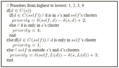
![\includegraphics[width=1.55in]{fig/avg_routing_stretch.eps}](fig3.png)
![\includegraphics[width=1.55in]{fig/dht_only.eps}](fig7.png)
![\includegraphics[width=1.6in]{fig/obstacle.eps}](fig8.png)
![\includegraphics[width=1.8in]{fig/sf/ll_suc.eps}](fig9.png)
![\includegraphics[width=1.8in]{fig/sf/ll_hop.eps}](fig10.png)
![\includegraphics[width=1.8in]{fig/sf/ll_tx.eps}](fig11.png)
![\includegraphics[width=1.8in]{fig/sf/ll_con.eps}](fig12.png)
![\includegraphics[width=1.8in]{fig/sf/ly_mem.eps}](fig13.png)
![\includegraphics[width=1.8in]{fig/sf/ll_ns_tx.eps}](fig14.png)
![\includegraphics[width=1.8in]{fig/sf/ld_ll_knb_data_suc.eps}](fig15.png)
![\includegraphics[width=1.8in]{fig/sf/ld_ll_knb_data_hop.eps}](fig16.png)