|
NSDI '06 Paper
[NSDI '06 Technical Program]
Practical Data-Centric Storage
Cheng Tien Ee
-
UC Berkeley
Sylvia Ratnasamy
-
Intel Research, Berkeley
Scott Shenker
-
ICSI & UC Berkeley
Abstract:
Most data retrieval mechanisms in wireless sensor networks adopt a data-centric approach, in which data is identified directly by name rather than through the location of the node on which it is stored. Initial data-centric methods, such as directed diffusion and TinyDB/TAG, focused on the conveyance of data.
One of the advantages of these algorithms is that they do not require point-to-point routing, which has proved to be difficult and costly to implement in wireless sensor networks, and instead require only the simpler and more robust tree-construction primitives.
Some recent data retrieval proposals have extended the data-centric paradigm to storage. Data-centric storage uses in-network placement of data to increase the efficiency of data retrieval in certain circumstances. Unfortunately, all such proposals have been based on point-to-point routing, and therefore have faced a significant deployment barrier.
In this paper we hope to make data-centric storage more practical by removing the need for point-to-point routing. To that end, we propose pathDCS, an approach to data-centric storage that requires only standard tree construction algorithms, a primitive already available in many real-world deployments. We describe the design and implementation of pathDCS and evaluate its performance
through both high-level and packet-level simulations, as well as through experiments on a sensor testbed.
1. Introduction
Deployments of wireless sensor networks (WSNs) in
recent years have grown steadily in their functionality and scale [25,31,1,13,3,18,34], but they still operate
under extreme energy constraints. Hence, the ability to efficiently extract relevant data from within the WSN remains paramount.
In their seminal paper [6], Estrin et al.
argue that efficient data-retrieval in WSNs requires a paradigmatic shift from the Internet's node-centric style, in which the basic communication abstraction is point-to-point (or multipoint) delivery, to a data-centric approach in which query and communication primitives refer to the names of sensed data rather than the identity (e.g., network address) of the sensing node.
The first generation of data-centric methods addressed the conveyance of data through the network. Directed diffusion [14], the first such proposal, determined data routes (and rates) based on reinforcement feedback from upstream nodes, resulting in tree-like data paths from the various sensing nodes to the base station (by which we mean the source of queries). A later method, TinyDB/TAG [23,24], explicitly constructs a delivery tree and then performs various forms of data manipulation as the data is conveyed to the base station.
A later generation of data-centric methods, inspired by the use of Distributed Hash Tables (DHTs) in the Internet, has focused on the storage rather than the conveyance of data. These solutions use intelligent in-network storage to make data retrieval more efficient.
In data-centric storage, sensed data are stored, by name, within the network. All data with the same name are stored at a single node, so queries can be routed directly (rather than flooded) to the node that stores the desired data.
Data-centric storage (DCS) can be used to support
a variety of sophisticated query primitives
such as multidimensional range queries [22,11], multi-resolution
queries [10], and approximate queries [12].
However, there has yet been any deployment in sensornets, though there are multiple scenarios in which they will be useful. For instance, we can imagine a sensor network deployed in a safari, monitoring the location of the various animals. Rather than querying each node to determine if it has seen an elephant, we can instead query a single node that is responsible for all elephant sightings.
These two classes of methods, data-centric conveyance and data-centric storage, have very different performance characteristics in terms of the energy expended to get the desired data. As discussed in [30] for the simplest cases of data-centric conveyance and storage, their relative performance depends on the nature of the data generation, the query rate, the network size, and many other factors.
More to the point of this paper, these two classes of methods require very different communication primitives from the network. The various data-centric conveyance methods rely (either implicitly or explicitly) on tree-construction techniques. Note that even the simplest method of data conveyance, whereby all data are proactively sent to the base station immediately upon generation, also relies on a spanning delivery tree.
Tree-based routing is both algorithmically simple and practically robust,
leading to its adoption
in a number of real-world deployments.
For example, simple proactive data delivery
was used in the deployments on Great Duck Island [25,31] and Intel's fabrication unit [3], while TinyDB is used in the deployments at the UCB botanical gardens [18].
In contrast, all known data-centric storage methods rely on a point-to-point routing primitive:
they deterministically map the name (say x) of
a data item to the routable address (say i) associated with a particular node. Node i is then responsible for storing all data named x and
all queries for x are routed directly to node i, thereby requiring point-to-point routing.
However, as we review in the following section, achieving scalable
and practical point-to-point routing is a difficult challenge.
While a number of recent research efforts [27,28,17,20,11,8] have made significant progress towards this end, point-to-point routing still requires significantly more overhead and complexity than tree construction as we will explain in the following section, and has yet to be used in real-life deployments. It thus seems unwise to couple data-centric storage to such a burdensome underlying primitive, particularly one that is not widely deployed. If data-centric storage is to become more widely used, it should rely only on currently available, and easily implementable, communication primitives.
Our goal is not merely to find a better algorithm for data-centric storage. More fundamentally, we hope to make data-centric storage a basic primitive available to WSN applications, and we recognize that this can only happen if data-centric storage is implemented with minimal assumptions about the underlying infrastructure.
To that end, this paper proposes a data-centric storage method called pathDCS that uses only tree-based communication primitives. The design relies on associating data names with paths, not nodes, and these paths are derived from a collection of trees. We investigate some basic performance issues, such as load balance, through high level simulation but for a more real-world evaluation we implemented pathDCS in TinyOS and report on its performance
in packet-level TOSSIM[21] simulations as well as in experiments on a mote testbed. To the best of our knowledge, this is
the first evaluation of a working prototype of data-centric storage.
Our results show that pathDCS achieves high query success rates (on our 100-node
testbed, we see roughly a 97% success rate) and is robust to node and network
dynamics.
Finally, we note that in this paper we only consider the basic
exact-match storage primitives as explored by schemes
such as GHT [29] and GEM [27]. We leave for
future work its possible extension to supporting the
more complex query primitives from the literature [22,12,10,9].
2. Background
The value of pathDCS relies on four basic points:
- Data-centric storage is a valuable paradigm in WSNs.
- Current data-centric storage techniques rely on point-to-point routing.
- Point-to-point routing is difficult, and imposes significant overhead on WSNs.
- pathDCS provides a scalable and robust implementation of data-centric storage that does not require point-to-point routing.
The bulk of this paper is devoted to demonstrating the fourth point. In this section, we briefly review the literature supporting the first three.
Data-centric storage (DCS) was first explicitly proposed in [30]. Analysis of a simple model identified scenarios in which DCS
outperforms the other data retrieval approaches, namely external storage (in which all sensed data is proactively sent to the base station) and data-centric routing (in which queries are flooded and only
relevant data are transmitted to the base station). This same analysis also identified scenarios where the other two methods outperformed DCS. Thus, DCS and other techniques should be seen as complementary, not competitive; our assumption is that DCS is a valuable method of data retrieval in some but not all circumstances.
Reference [30] presented only the simplest form of data-centric storage: an exact-match query-by-name service where the named data can be directly retrieved. A number of subsequent proposals extend the idea of data-centric storage to support more
complex queries such as multi-dimensional range queries [22,11], multi-resolution indexing [10] and spatially distributed quadtree-like indices [12].
Data-centric storage requires a hash-like interface where data (or data structures) can be stored and retrieved by name. In all the above proposals, this is achieved by deterministically mapping (typically by hashing) a data name to a geographic location within the network. The node geographically closest to the hashed location is deemed responsible for storing information associated with the hashed name; geographic
point-to-point routing is then used to reach this storage node.
While elegant in structure, this approach requires that nodes know the
network's external geographic boundary so that names are mapped to geographic locations within the network. If they don't, most data will end up stored by edge nodes, after an extensive perimeter walk, resulting in uneven load and inefficient operation. The various proposals acknowledge, but do not address, this challenge.
The original geographic routing
algorithms such as GPSR (see [2,16,19]) were designed for unit-disc
connectivity graphs under which a node hears transmissions from another node if and only if they are
within a fixed radio range. (This assumption is crucial for the perimeter walk phase, but is not needed for the greedy phase of geographic routing.) Measurements have shown that
this assumption is grossly violated by real radios [33,35,8]
and that geographic routing breaks down in such cases [17].
In recent work, Kim et al. [17]
and Leong et al. [20] proposed extensions to GPSR
that removes the need for the unit-disc assumption.
CLDP [17] represents a fundamental
breakthrough in that it guarantees correct operation over
topologies with even arbitrary connectivity. GDSTR [20] on
the other hand routes on spanning trees when greedy forwarding
is unable to make progress. In both cases additional complexity
and overhead is required.
An even more basic assumption underlying geographic routing is that each node knows its geographic coordinates.
While some sensor nodes are equipped with GPS, the widely-used Berkeley mote
is not: although other localization techniques do exist, none
of them have been evaluated for their potential to serve as
routing coordinates. Motivated by this challenge, GEM [27] and
NoGeo [28] explore the construction of virtual coordinate
systems; these are synthetic coordinates to which geographic routing can be applied. Like CLDP, GEM and NoGeo represent
significant conceptual advances but come at the cost of increased
complexity. NoGeo requires O(N) per-node state during initialization
while GEM can incur significant overhead
under node and network dynamics.
Finally, there are a number of proposals for point-to-point routing
in the literature on ad-hoc wireless networks.
Many of these solutions face scalability problems when
applied to wireless sensor networks and are thus unlikely to serve
as a substrate for DCS. We refer the reader to [8] for a more
detailed discussion of the space of point-to-point routing
algorithms and their applicability to WSNs.
As the above discussion reveals, there has been
significant progress on point-to-point routing for WSNs and
both BVR and CLDP have resulted in working implementations
for the mote platform.
At the same time, the various solutions remain fairly
complex (at least relative to tree construction) and face further
challenges in supporting in-network storage.
For these reasons, we deemed it worthwhile to explore
an alternate approach that releases DCS from the challenges and
complexities of point-to-point routing.
3. Design
We begin this section with the description of the core pathDCS
algorithm, followed by those of supporting ones.
3.1 Core Algorithm
For pathDCS to be effective, it must be consistent: that is, all queries and stores for the same object (no matter from where they are issued) must reach the same destination. The traditional way to ensure consistency is to give all nodes a shared frame of reference that allows packets to describe their destination and enables forwarding nodes to route packets to that destination.
We use a few shared points of reference called landmarks (places with well-known names that all nodes can reach), and name locations by their path from one of these shared points of reference [32]. For example, when giving driving directions (in real life) we often use a well-known landmark and then provide path-based instructions: ``Go to the gas station, and then take your first right, and then after two blocks take a left...." The driver need only know (a) how to find the landmarks and (b) how to follow a set of procedural directions. This is the approach used in pathDCS. We map each name to a path, not a node, and that path is defined by an initial landmark and a set of procedural directions that are defined in terms of other landmarks. To query or store that name, a packet goes to the designated landmark and then follows a set of procedural directions; the store or query is then executed at the node on which the path ends. Notice that the end-point of the path is independent of where the query or store is issued from; since the path starts off by going to a particular landmark, its origin doesn't matter.
In pathDCS the landmarks are a set of beacon nodes, which can be elected randomly or manually configured (see Section 3.2). To make sure that all nodes know how to reach the beacons, we use standard tree-construction techniques to build trees rooted at each one of these beacons. The overhead to establish the necessary state is proportional to the number of beacons; as we will see, that number is small so pathDCS imposes little overhead.
The paths are specified in terms of an initial beacon and a set of segments, with each segment consisting of a direction (defined in terms of a beacon) and a length (defined by how many hops). Thus, each path consists of a sequence of p beacons bi and lengths li, where
i = 1,..., p.1 The packet is first sent to beacon b1. From there, it is sent l2 hops towards beacon b2 using the tree rooted at b2. The process then repeats; from wherever the packet ended up at the previous i - 1 segment, it is then sent li hops towards the next beacon bi. The path ends after the pth segment.
To make this more precise, we first define some terms. There is a linear space of identifiers, say 16-bit addresses, that is large enough so that there are no clashes in identifier assignments. Each node in the network is assigned a logical identifier id.
Data is associated with a key k (assume this is derived from a hash of its name) and, for node n, the hop distance to beacon b is given by hops(n, b). Let ni denote the identifier of the node on which the ith segments starts (also the place where the previous segment ends). Lastly, there is some hash function h(k, i) which maps an identifier k and an integer i into an identifier.
When accessing a data item with identifier k, the set of beacons used for the path are determined by consistent hashing [15]: beacon bi is the beacon whose identifier is closest to (in the sense of consistent hashing) the identifier h(k, i). In addition, the first segment length l1 is always equal to the distance to the first beacon b1, whereas segment lengths for i > 1 are given by:
| li = h(k, i)modhops(ni, bi) |
(1) |
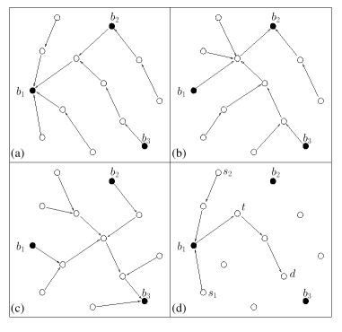
Figure 1:
(a), (b) and (c) show the routing trees rooted at beacons
b1, b2 and b3 respectively. (d)
Source nodes s1 and s2 both send packets with the same
key. These packets first reach a common first beacon (b1), before taking
the same subsequent path segments to reach destination node d.
|
We use Figure 1 as an example to illustrate how pathDCS routes packets with the same key from different source nodes to the same destination node.
For clarity we show the routing trees rooted at b1, b2 and b3
in Figures 1a, 1b and 1c
respectively.
We fix the total number of path segments at 3, and
both source nodes s1 and s2 generate packets with the same key k.
Both the current number of remaining hops and the current path segment
i (also called segment counter)
are carried in the packet header and modified as needed.
In the figure, beacons b1, b2 and b3 are chosen because their ids are closest to h(k, 1),
h(k, 2) and h(k, 3) respectively. The order of beacons towards which packets
are forwarded is therefore b1, b2 and b3, following the order of
segments traversed. Initially, both packets are routed
to b1, upon which it is determined, using Equation 1,
that in the second segment they should be
forwarded towards b2 for, say, 1 hop. At node t, which is the terminating node
of the second segment, the segment counter in the packet header is incremented,
the number of hops is again computed using Equation 1 (assume the result is two),
and the packets are subsequently forwarded two hops towards the third
and final beacon, to terminate at node d.
Node d is then the destination node for all data associated with key k.
The number of hops required for each query or store is proportional to the diameter of the network, which is the same for all DCS approaches, multiplied by the number of segments. Thus, the key to keeping the overhead of pathDCS manageable is keeping the number of segments, p, small. As we argue below, p = 2 is sufficient for reasonably-sized networks, so that we expect the per-query expenditure to be a few multiples bigger than in other DCS schemes.
The pathDCS algorithm has two parameters: B, the total number of beacons and p, the number of path segments. Varying B trades off the control traffic overhead due to tree construction versus load on the beacons. We explore this
tradeoff in Section 5. With regards to p, increasing
the number of segments results in longer paths but potentially spreads the storage
load more evenly. To see this how large p should be to achieve reasonable load distribution, consider the following naive
back-of-the-envelope calculation. The total number of paths a
message can traverse using pathDCS is approximately Bp. Letting d be the network density and r the radio range, the expected length of each path is given by
 |
(2) |
Thus the number of nodes pathDCS routing can potentially use to store data is
approximately
 |
(3) |
Equating 3 to total number of nodes N, the number of
beacons required is given by
 |
(4) |
As an example, we plug in the following values: r = 8 units, d = 0.07 nodes
per unit area,2N = 20000, and for p = 2, we obtain
B &asymp 24, which is a reasonable number.
We did simulations for
p = 2, 3, 4, 5
to verify that indeed the distribution of load changes
very little with increasing p and then picked p = 2 since it, as expected, resulted in the shortest paths. Note that knowledge of N by every node is not required, only
p and B need be set at deployment. Unless the network size changes
drastically we do not expect performance to degrade significantly.
3.2 Supporting Algorithms
While the basic idea of pathDCS is contained in the core algorithm defined above, actual implementation of pathDCS requires a set of supporting algorithms to, for example, select beacons and build trees. There is nothing novel in these algorithms, we describe them for completeness.
To construct a tree rooted at a particular beacon, we recursively have nodes pick a parent that is closest to that beacon amongst all their neighbors. Our implementation uses the ETX [5], also the MT [33] metric as an indication of path quality.
The total number of beacons in the system is a fixed
constant B, and is dependent on the size of the network. We divide the identifier
space into B equal partitions, and have each node compete to become the beacon for the
partition in which they reside. Borrowing the basic concept from SRM [7],
each node's self-election announcement is delayed by time proportional to the
difference between their ids and the largest identifier for that partition (i.e.
the identifier that describes the upper boundary of that partition).
For instance,
if we assume that B = 4, and node X, Y and Z's
identifiers fall within the partitions 2, 2 and 4 respectively,
only X and Y compete to be the beacon in partition 2.
X and Y independently set a timer
with delay
(I2 - idX) and
(I2 - idY) respectively, where I2
is the largest possible identifier for that partition, and is some
constant. This scheme ensures that
node Y, with the higher id, usually announces itself before X,
thereby suppressing X's announcement.
It is possible that the election process results in two or more beacons clustering.
An additional rule can be imposed to reduce the occurrence of this scenario: when
timeout occurs and just before a node announces itself as a beacon, it checks to
see if any beacons lie within k hops. If so, it suppresses its announcement.
From time to time, the role of beacons should be handed over to other nodes,
either due to failures, or to reduce the forwarding load on the beacons.
In the case of the former, one hop neighbors begin a self-election process
once the link quality to that beacon drops below a threshold. Similar to the
initial election process, the delay for the timer set is a function of the
difference between the current node's identifier, and that of the
highest identifier for that partition. Note that in this case all one-hop
neighbors participate in the election. The winning node then takes over the
identifier of the deceased beacon, and assumes that role henceforth.
For the case of deliberate handoff, the beacon randomly picks a neighbor, and switches
identifiers with it.
Possible different criteria exist, the meeting of any one can
trigger deliberate handoff. An example of a criterion would be a minimum
amount of remaining energy. In this case, the time at which handoff is
triggered is very much dependent on the rate at which the application
generates data packets. One can also imagine the beacons handing off in order
to spread themselves out if they are clustered together.
The proximity of the current and previous beacon ensures that drastic route updates
in the network are minimized. Specifically, the destination nodes for a particular
key before and after the handoff takes place should lie close to each other, in
terms of number of hops. Together with data replication mentioned below,
this increases the chances of finding the data before
the next data refresh (see below) or before new data is stored at the updated location.
In the typical case, where the querying node is the base station (or any other well-defined node), we construct a tree rooted at that node. Answers to queries are sent back along this tree to the base station. If queries are being issued from multiple nodes, then each such node includes its closest beacon in the query. Backward path establishment from that beacon is performed by storing pointers to the previous node at each intermediate hop. Responses to queries are sent back to the closest beacon (as noted in the query) and that beacon forwards the response along the path that was established from the querying node by the path establishment message.
Every node where data is stored will periodically issue refresh probes for those data. These probes are routed in the same manner as the data packets, allowing the node to detect if the topology has changed since the initial storing.
If the node initiating the refresh does not receive the probe in return, it then stores the data at the new location.
Finally, local replication of data is performed at the storage node. Data packets are disseminated using a localized flood within k-hops of the destination. A query reaching a destination not storing the required data is similarly flooded locally, with replication nodes responding to the query.
4. Performance Metrics
Before proceeding to the sections on simulation and
implementation details and results, we elaborate on
the metrics of interest, namely
path consistency, storage and forwarding load balance.
The design of pathDCS raises three performance questions.
The first has to do with the consistency with which pathDCS
maps names to storage locations. In the absence of node and
network dynamics, pathDCS achieves perfect consistency in that
stores and lookups for a particular data item always terminate
at the same storage node, and hence pathDCS would see a 100%
success rate for lookups.
However, node and network dynamics can lead to changes
in the paths to beacons and hence to changes in the mapping
between a name and storage node. The extent
to which such changes impact lookups depends
on both the frequency and the extent of changes.
If changes in storage nodes are highly localized, then
simple local replication of data should trivially mask such changes.
If changes are infrequent, then a periodic refresh of stored data
should suffice to maintain high success rates. In any case,
pathDCS provides only weak consistency: it does not guarantee that
the data retrieved is the latest stored.
These path changes are primarily dependent on the behavior
of the wireless medium and hence we explore this issue in detail
in Section 6. However, such changes are also dependent on network size because longer paths are more likely to experience changes. Since we can't analyze scaling effects on our testbed, we use an idealized, but highly pessimistic, model of path dynamics in our simulator to see how consistency varies with system size. To quantify consistency, we measure the lookup success rate, which is the probability that a lookup for a data item x reaches a storage node currently storing x.
To understand
the magnitude of lookup variations,
we also measure the maximum separation in hops
between any two nodes storing a particular data item,
which we call the spread. This measures the extent to which local replication can mask the effect of path dynamics.
The second performance issue has to do with how effectively pathDCS balances the
storage and forwarding load across nodes.
This is a potential issue because unlike other DCS schemes that
explicitly distribute data items over the set of all nodes, pathDCS
distributes data over a more limited number of paths.
While we do not expect pathDCS to achieve load distribution comparable
to the address-based DCS schemes, we would like to verify that
the load distribution in pathDCS is not unreasonable.
5. High-Level Simulation Results
5.1 Overview
The performance of pathDCS derives from the inherent
behavior of its algorithms as well as
the impact of the wireless medium on both
the algorithms and our particular implementation choices.
To separate the effects of each, we
evaluate pathDCS through a combination of
high-level simulations (to evaluate the scaling behavior
of the algorithms themselves),
low-level simulations
that take into account a lossy medium and packet collision effects,
and implementation (to
evaluate pathDCS under realistic wireless conditions).
This section presents our high-level simulation results;
our prototype and its evaluation in TOSSIM [21] and on actual
testbeds are described in Section 6.
Our simulator makes a number of simplifying assumptions
that abstract away the vagaries of the wireless
medium. Nodes are placed uniformly at random in
a square plane and every node is assigned a fixed circular
radio range. A node can communicate with all
and only those nodes that fall within its radio range.
In addition, the simulator does not model network congestion
or packet loss. While clearly unrealistic, these simplifications
allow simulations that scale to thousands of nodes; our
packet-level simulation and testbed
results in the following section capture performance under
more realistic conditions.
Our default simulation scenario uses 5000 nodes
placed in an area of
6.7 x 10⁴ units2 with
a radio range of 8 units, leading to an average node
degree of 14.5. We maintain the same density for all simulations.
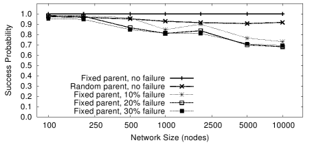
Figure 2:
Success rate under failure and randomized parent selection
for increasing network sizes. All tests use 20 beacons and 2 path segments.
|
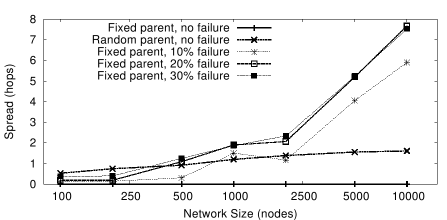
Figure 3:
Spread under failure and randomized parent selection
for increasing network sizes. All tests use 20 beacons and 2 path segments.
|
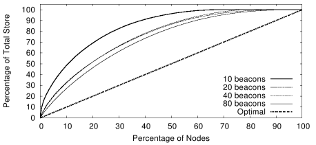
Figure 4:
CDF of storage load with pathDCS and
``optimal'' DCS for different numbers of beacons.
|
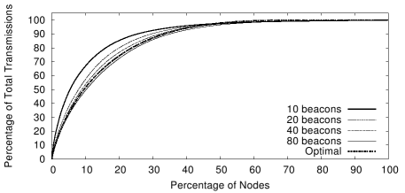
Figure 5:
CDF of transmission load with pathDCS and
``optimal'' DCS for different numbers of beacons.
|
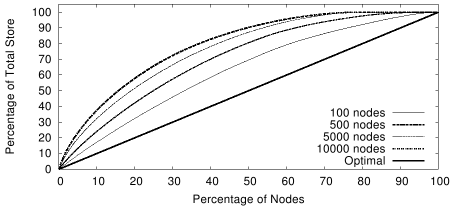
Figure 6:
CDF of storage load using pathDCS for
increasing network sizes.
|
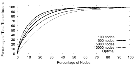
Figure 7:
CDF of transmission load using pathDCS
for increasing network sizes.
|
5.2 Lookup Success Rates
The path to a beacon can change for two reasons: (1) tree reconfiguration following node
failure(s) and (2) variations in link
quality that trigger a change in a node's choice of parent. The first we can accurately model in simulation, the second we can only roughly approximate.
We perform the following test to measure success rates: for
a network with N nodes, every node inserts 10 distinct data
items into the network yielding a total of
10 x N distinct
data items. Stores are replicated within the one-hop neighborhood
of the destination. We then perform 20 lookups
for each data item. A lookup succeeds if it arrives at a node
storing the requested data item (either at the original destination, or at one of the one-hop replicas); otherwise, the lookup
fails.
To measure spread, we repeat the same tests as above but now we
turn off one-hop replication and have each node
store (rather than lookup) every data item 20 times.
For each data item, we then consider the set of nodes storing
that item and measure spread as the maximum separation in
hops between any two nodes in the set.
To capture the effect of node failure, after each
of the 20 iterations for a given item, we
fail a fixed fraction of nodes uniformly at random
and then recompute the trees for each beacon.
Capturing varying link qualities is more problematic because
our simulator does not model congestion and packet loss;
instead, we directly address the effect on parent selection.
We conservatively model changes in parent selection arising
from varying link qualities as follows:
rather than pick a single parent for
each beacon, a node considers
all of its neighbors that are closer to
the destination beacon than itself as potential
parents. For every message, a node then chooses
its next hop uniformly at random from this entire
set of potential parents. This represents a highly
pessimistic scenario in which, at every hop, the route
to a beacon can flap between all possible next-hops.3
Recall that fixed parent selection with no failure has a success
rate of 100% and a spread of zero since we turn
off one-hop replication when measuring spread.
Figures 2 and 3 plot the
average success rate and spread under
increasing network size using random parent selection
or fixed parent selection under various failure rates.
As expected, we see that the success rate drops, and
spread rises with network size but this deterioration is slow.
For example, a 10,000 node network with random parent selection
(which, again, is a pessimistic model)
still sees a success rate of 92%.
Moreover, the absolute value of spread is often
low and hence could frequently be masked by simple k-hop local
replication. We implement just 1-hop replication but for
very large networks (>10,000 nodes) with high failure rates (30%)
one might need a larger scope of replication.
Section 6 continues this evaluation in
real wireless environments.
5.3 Load Distribution
There are only two knobs to the basic pathDCS algorithm: (1) the
total number of beacons and (2) the number of path segments used.
Ideally, we want to pick a number of beacons and path segments
that allow forwarding and storage load to be well spread out
while maintaining reasonable path stretch.
The analysis in Section 3 leads us to the choice
of 2 segments and hence we now look at the number of
beacons required to achieve good load distribution.
We first hold N, the network size, fixed
at 5000 nodes and scale B, the number of beacon nodes.
As before, every node uses pathDCS to insert 10 distinct data items
into the network yielding a total of 50,000 distinct stored items.
We then measure the per-node forwarding and storage load.
Figures 4 and 5
plot the cumulative distribution function (CDF)
of the storage and transmission load respectively.
To determine if any load imbalances are due to pathDCS, or are inherent
in the DCS approach, we also plot the distributions for an ``optimal'' form
of DCS in which names are mapped uniformly at random over
the entire set of nodes and stores follow the shortest
path from the inserting node to the destination storage node.4
In terms of storage, we see that usage of just 20 beacons
results in a fairly even distribution and that increasing
B beyond 20 offers rapidly diminishing returns.
In terms of transmission load, we see that the pathDCS distribution
approaches that of the optimal although both are
fairly skewed.
This is due to the natural concentration of traffic
in the center of the grid and is in no way
specific to pathDCS or even DCS schemes in general; rather this is
an issue for communication in all ad hoc networks
and one that has received some attention in the
literature [26].
At less than 1% of the total number
of nodes, B = 20 represents very low control overhead in
terms of tree construction. Moreover, we see that the pathDCS
distributions are reasonably close to the optimal node-based DCS.
Given the relative simplicity of pathDCS, this seems
like a very worthwhile tradeoff.
We now investigate the variation of performance with increasing
network size. We fix
B = 20 and scale N.
Figures 6 and 7 plot the
CDF of transmission and storage load respectively. We
see that, as expected, the distribution deteriorates with
increasing N but this deterioration is very gradual.
Finally, the stretch in all our tests was approximately
2.4 which is in keeping with our use of 2 path segments.
We also verified that stretch increases as we increase
the number of path segments.
In summary, this section explored the basic scaling behavior
of the pathDCS algorithms. We show that pathDCS is robust
in that it achieves high success rates under highly pessimistic
models of node and network dynamism. Moreover, pathDCS
is scalable in that it requires a small number of beacons
to achieve good load distribution.
6. Implementation Details and Results
We implemented pathDCS in TinyOS, and evaluated its performance
on the 100-node Intel Mirage [4] micaZ testbed as well
as on 500 nodes in TOSSIM's packet-level emulator.
We begin this section by briefly describing the pathDCS system architecture,
followed by low-level details of the implementation in TinyOS, and finally
ending with evaluation of its performance.
6.1 PathDCS System Architecture
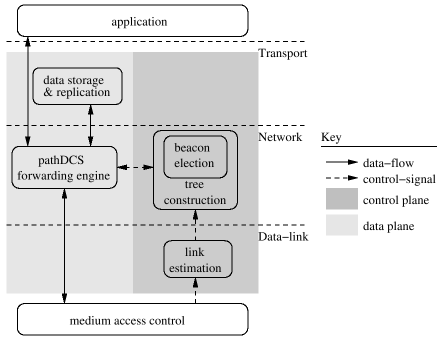
Figure 8:
The pathDCS architecture is made up of
(1) the data plane, consisting of the forwarding engine and data storage
and replication component, and (2) the control plane, consisting of the tree
construction and related components.
|
Figure 8 shows the pathDCS system architecture, which can be
divided into control and data planes.
The control plane provides primarily beacon election and tree-based
routing capability, whereas the data plane implements the core pathDCS
forwarding logic (using the control plane's tree-based routing tables),
storage of name-value pairs, and one-hop replication. Note that
the only component specific to pathDCS is the forwarding engine;
the remaining components are common to a number of other systems
such as TinyDB [24] and BVR [8].
6.2 Control Plane
We next elaborate on the implementation of the control plane.
This component primarily constructs trees rooted at the beacons, disseminating
and maintaining information used to determine the next hop at every
node for each beacon in the network. We begin by describing the network-wide
naming mechanism.
Each node in the network is assigned a hardware address5 that is unique in the
sensornet. This address is subsequently hashed to obtain the corresponding
network identifiers. Since the hash function is known, collisions
can be avoided by setting the hardware addresses appropriately.
Periodically, each node broadcasts distance vector packets containing
the identifiers and distances to each beacon in the network. If the
relevant element in the vector indicates a beacon in the same partition
with a smaller identifier, a node elects itself by replacing the identifier
with its own before broadcasting. In this manner, the entire network
eventually learns the beacons and their corresponding identifiers.
Nodes periodically broadcast estimates of their neighbors' reception qualities
within their immediate neighborhood, allowing these neighbors to compute the
link quality in both directions, thus accounting for asymmetric links. Messages are
jittered slightly at each node to minimize interference.
The link estimator module maintains, for each neighbor, a periodically
updated estimate of link quality, which is the
expected number of transmissions to that neighbor. This is
computed as an exponentially weighted moving average:
Lav, i = (1 - &alpha)Lav, i-1 + &alphaLi
where Lav, i and Li are the average
and sample respectively for iteration i and &alpha is a constant.
Only route update packets are used as samples for the computation.
Beacons periodically generate routing updates which are
propagated through the network in a distance vector manner.
A node uses the beacon election rules
described in Section 3 to decide whether it
should elect itself as a beacon.
Nodes use these route updates to compute their minimum ``distance''
to each beacon. To reduce transmission loss, we use the MT [5],
or ETX [33] metric,
where the number of expected transmissions
to each beacon is minimized.
Control messages broadcasted by a node include information such as
its current hop distance and estimate of the expected number of
transmissions to
each beacon, the latest sequence numbers associated with the corresponding
beacon, and the node's estimate of its
neighbors' reception qualities. To remove the occurrence of one-hop count-to-infinity
problems, control packets also include the next hops for each beacon, so that
a node does not attempt to forward packets to its neighbor which will subsequently
forward the packet back.
6.3 Data Plane
In this paper, the data plane operations of interest
include the forwarding of pathDCS data packets and their replication.
The description of these operations is followed by an brief coverage
of the packet header overhead.
Packet headers include fields that contain the key and the current
path segment the packet is on. Based on routing information provided by the
control plane, these are used to determine the next
beacon to route towards and the number of hops to take, as
elaborated in Section 3.1.
The remaining hops before reaching
the end of a segment is also carried in the header.
Replication of data to improve availability is achieved
by scoped flooding once the data packet reaches its destination node. The field
previously used to indicate the number of remaining hops is used
to specify the scope of the flood, and is decremented with each subsequent broadcast.
To prevent repeated broadcasting of the same packet in the local neighborhood of a
node, a cache of the most recently sent ones is kept.
The overhead incurred in each data packet is small. In our implementation, pathDCS
uses 6 bits to represent the key associated with each data type, thus allowing for
a total of 64 keys.6
In general we expect the number of unique data types to be small
and independent of the size of the network. Also, in the case where the number
of path segments is 2, we require an additional bit to keep track of the current
segment the packet is on. Finally, the remaining hops to the terminating node of
the current segment is also stored in the header, and is on the order of O(logD),
where D is the maximum diameter of the network. In our implementation, the total
number of control
bits used to route data is just
(data + segment + hops) = 6 + 2 + 8 = 16 bits.
6.4 Methodology
The primary concern when implementing pathDCS is the impact of its
dependence on path stability. Whilst the construction of routing trees
had been studied extensively, the main focus in previous studies
was the successful forwarding of packets to the destination. Of little or no
significance were the paths along which data packets traverse as long as they
can get there. In pathDCS,
the destination node is effectively defined as a function of the network's
current routing state. As a result, if the network state changes frequently, we may
store and query data items at destinations that shift rapidly
with time. Such a situation will result in poor lookup success
rate, rendering pathDCS less useful. This is therefore the most important
point to address in our implementation.
Thus, as in Section 5, we are primarily
interested in the probability of lookup success. A lookup can fail either
because the message was dropped along the way,
or because the destination node it arrived at did not
have the requested data. Two metrics are used to distinguish between
these two causes.
The first is the route completion probability, measured as
the probability that a packet successfully arrives at a destination node
(as opposed to being dropped along the path). Note that the
route completion probability has little to do with the
pathDCS algorithms per se. Instead, such failures are
dependent primarily on the characteristics of the wireless
medium and our implementation choices for the
link estimation, tree construction and retransmission modules.
In general the quality of links in the network fluctuates over time, resulting
in route updates as the network attempts to pick routes that result
in lower loss.
The second performance metric is our usual lookup success rate as
defined in Section 4. In computing this rate,
we consider only those lookups that complete
(that is, they reached some destination node), and we say that a lookup
is successful if it locates the requested data item.
To measure the effect of variable node and network conditions,
we obtained the lookup success rate for different values of
data refresh intervals. This is achieved as follows:
in each experiment, we have
all nodes periodically route some number of messages for each distinct
data item. For the routes that do complete, we then observe
where those messages terminate.
Next, we divide time into windows, where the first data packet in
that window is treated as a store or refresh packet,
and the node at which it terminates
is the storage node for that window. Subsequent packets then act
as queries and lookup success is measured as the
probability that a lookup arrives within the
one-hop neighborhood7
of the storage node for that window. We do this for each distinct
data item, compute the average lookup success and repeat
for different window sizes.
We note that varying this window size is equivalent to altering
the data refresh interval, and we can thus use a single experiment
to observe the effect of increasing refresh intervals
rather than running repeated experiments that may suffer from
different time-of-day effects.
Data refreshing plays a crucial role in improving lookup success,
especially in large networks (of size in the hundreds to thousands),
where the path may vary widely over time.
When we consider short time-scales,
say within a period of a minute or two, the set of destination nodes for
a particular key is probably small in number, and
not likely to be spread out over a large region.
However, when looking at all possible destinations over a period of a
day, the set of nodes will be the union of all sets at shorter time-scales:
it is more likely to be large, as well as covering
a wider area. Thus, a refresh rate that is high translates into
observation at small time-scales, which means that destinations are
close together, and therefore lookup success increases. We validate this
in the following sections, via simulation and experiments on the testbed.
6.5 TOSSIM Simulations
In this section we describe packet-level simulations
that model a lossy medium. A total
of 500 nodes were simulated using actual TinyOS code. We
begin by elaborating
on the parameters used in the simulations as well as in the testbed's motes.
Table 1:
Control plane parameters
|
Parameter Description |
Value |
|
Number of beacons |
5 |
|
Distance vector (DV) broadcast interval |
10 seconds |
|
Maximum DV broadcast jitter |
1 second |
|
Frequency of route updates |
1 per 10 DV pkts |
|
Maximum entries in neighbor table |
16 |
|
Moving average for link estimation, &alpha |
0.05 |
Table 2:
Data plane parameters
|
Parameter Description |
Value |
|
Number of path sections |
2 |
|
Scope of flooding for local replication |
1 |
|
Maximum retransmissions to the next hop |
5 |
|
Maximum cached replication entries |
4 |
The appropriate choice of parameters is dependent on the size of the network,
as well as the desired properties of the applications that run on it. For
instance, as we shall demonstrate in the subsequent sections,
stable paths are a prerequisite for high lookup success in pathDCS.
Stability can be improved by damping route updates at the
expense of increased network reaction time to topology changes.
Our choice of system parameters is shown in Table 1,
and has been experimentally verified to yield satisfactory performance.
The heart of pathDCS lies in the data plane.
Parameters associated with pathDCS can be tuned here,
and are largely independent of the control plane. As in Section 5,
we use only 2 segments in our implementation. This leads to
lower stretch, an important consideration in real networks
since longer routes result in an increase in loss probability. A shorter route is important also because it results in fewer
transmissions, which consume energy in resource constrained sensor motes.
Table 2 shows the parameters used in the data plane.
In each experiment, every node in the network generates different
data items, thus data destined for a particular destination node
originate from multiple sources. On average, data packets are
injected into the network at the rate of two per second to minimize
congestion. A total of 20 experiments are run, with each experiment
querying or storing a particular, distinct key, and each node
sending 72 packets. The network is allowed to run for a simulation hour
for routing to converge before queries and storage began.
With the above parameters, we measure
the route completion probability, the destination node spread distribution,
and the lookup success rate under two test scenarios:
we measure performance using the above default
parameter selection,
we look at the impact of our
choice of parameter selection on path stability and consequently
on pathDCS performance. Specifically, the parameters for this test are
the same as those for ``Normal''
except that the DV broadcast interval in Table 1 is reduced
to 5 seconds, and the corresponding maximum jitter to 0.5 seconds.
In general faster route adaptation can be desirable for reduced
recovery time from failures.
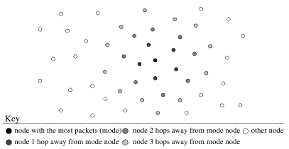
Figure 9:
The measure of destination spread distribution is based on the
hop distance from the node that received the most packets (i.e. the mode).
|
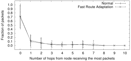
Figure 10:
500-node simulation: distribution of destinations for the
normal and fast route adaptation scenarios.
|
Since paths are likely to change over time, we need to
investigate the destination spread distribution.
Even though we expect the spread of destination nodes
to be significant, the situation is not hopeless if we find that most
of the packets still fall within a small region.
Using Figure 9 as an illustration,
we proceed as follows: we first determine the
node that received the most number of packets for a particular key, we
call this the mode node.
Then, for each hop from the mode node, we compute the total fraction of
packets that end on nodes at that distance. If the destination nodes
are evenly spread out over a wide area, then the distribution will show
a relatively flat graph over multiple hops. On the other hand, if the
nodes are highly clustered together, we should see a graph that peaks at
the 0th hop, with small fractions at the other hops.
In both scenarios, the mean network diameter is 18,
the average probability of route completion is about
86%,8
and the mean number of neighbors is around 10.4.
Figure 10 shows the distribution of destination nodes,
from which we can observe the following:
- The majority of packets (80%) land within one hop of the
mode node. This implies that, without data refreshing and with one hop
replication,
the mean probability of lookup success will also be about 80%. As we shall see
subsequently, data refreshing increases this probability. Another alternative
will be to increase the scope of local replication, which will however be
at the expense of more transmissions and storage space.
- Having more dynamic routing does not affect the resulting destination spread.
This is due to the fact that, over time, all possible combinations of routing
state, and correspondingly all possible destinations, have been encountered.
Increasing the rate at which changes occur does not affect this destination set.
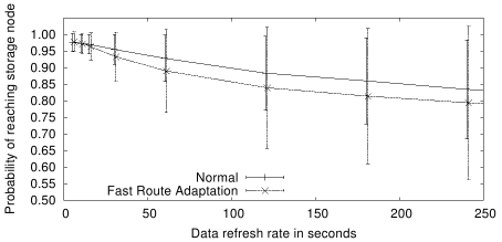
Figure 11:
500-node simulation: variation of lookup success with data
refresh interval.
|
We next consider the effect of data refreshing. As described in
Section 6.4, lookup success now refers to average fraction
of queries
that end within the replication region for all window periods. These
periods, or refresh intervals, are varied from 5 to 250 seconds, and the
results are shown in Figure 11. We can observe that
- Refreshing data more frequently can increase the probability of a
successful query to >95%.
- Faster route adaptation results in lower lookup success for a particular
refresh interval.
- Variation in lookup success is higher for routing that updates more frequently.
- As the refresh interval increases, lookup success probability approaches that
of packet fraction received within one hop of the mode node, which agrees with
Figure 10.
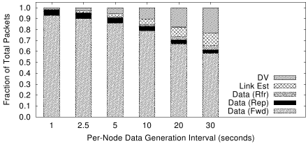
Figure 12:
500-node simulation: breakdown of transmissions for each packet type.
|
Finally, we consider the overhead incurred by pathDCS, focusing on the total number
of each type of packet transmitted. We identify five types of packets: (1)
distance vector (DV), (2) link estimation, (3) data packet
transmission for replication,
(4) data packet transmission for forwarding, and (5) data packet transmission for
refreshing. Figure 12 shows the breakdown for various
application data generation rates. We assume that the refresh per data type
occurs once every
100 seconds, and that there are 100 data types in the network. The rest of the
network parameters are as given in Tables 1 and
2. From the figure,
we see that the fraction of overhead packets reduces with an increase in application
rate, which is what we expect in general. Furthermore, the cost of refreshing data
is low, compared to the initial data replication and forwarding.
To summarize, the 500-node packet-level simulation shows that local replication by itself
is sufficient to result in high (80%) lookup success. Refreshing data periodically
counters the effects of routing changes, and is able to increase lookup success to (>95%).
However, the tradeoff is that more packets are transmitted, increasing the
overhead incurred.
We now proceed to evaluate the performance of pathDCS on the Intel Mirage testbed.
6.6 Testbed Details and Results
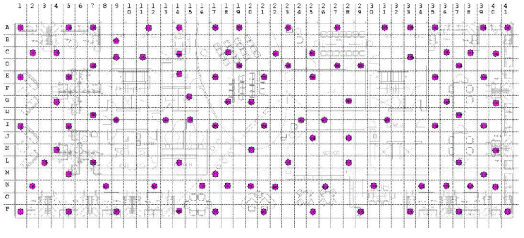
Figure 13:
Location of sensor motes of the Intel Mirage testbed is indicated
by the stars.
|
The Mirage testbed is located indoors, covering an entire floor of
the building. The 100 micaZ motes are spread out over an area of approximately
160' by 40', at the locations indicated in Figure 13.
Each mote in the testbed has a serial interface that
is connected to an internal ethernetwork,
which in turn is accessible via the Mirage server. Binaries are
uploaded and data downloaded via this ethernetwork, with the server
providing timestamping service for downloaded data packets.
We reduce the transmission power of the motes to reduce the effective
density of the network. For all our experimental results in this section,
the diameter of the network is 6.
Packet generation, test scenarios and network parameters are the same as that of
the packet-level simulations in Section 6.5.
For the testbed, the mean number
of per node neighbors is about 11.8, with the probability of route completion
being 97.9% and 96.1% for the normal and fast route adaptation
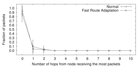
tests respectively. Figure 14 shows
the spread of the destination nodes for both test scenarios. We see that
in both cases the majority of packets terminate at a particular destination node,
87% for normal and 93% for fast route adaptation. If we consider all packets
that terminate within one hop of the mode node, this figure rises to about
97% in both cases.
Note that this takes into account all possible route changes and thus
destinations for the duration
of an experiment, and does not include the benefits gained from data refreshing.
Thus, it is clear that for the testbed of size 100, we can obtain high lookup
success even without refreshing.
Figure 14:
Distribution, or spread, of the destination node.
The fraction of packets landing x-hops away from the node with
the highest fraction is shown.
|
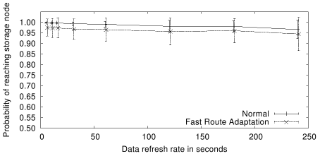
Figure 15:
Probability of lookup success for particular data refresh
intervals.
|
On the other hand, when we consider data refresh, a routing system
that is more dampened increases the chances of lookup success.
Figure 15 shows the corresponding lookup
success probabilities for these two systems. Four observations
can be made from the figure:
- The lookup success is very high in both cases even with low refresh
rates, which agrees with
the observation in Figure 14 that the set of possible
destination nodes is small.
- With increased damping, the system, in particular the paths,
are more stable, resulting in less variation in lookup success.
- For a given refresh rate, lookup is generally worse for
a more adaptive control plane.
- pathDCS constructed over a more dynamic routing control plane
has to refresh its stored data more frequently
in order to meet more stringent lookup success requirements.
In conclusion, the performance of pathDCS ultimately relies on the choice
of parameters at the underlying control plane.
Although the instability of paths causes the set of destination nodes
to increase, we find that in general they tend to be highly clustered,
with the majority of packets terminating on a small subset. Thus path
fluctuations
can be countered via two mechanisms: an increase in the scope
of local replication, or an increase in the frequency of data refreshes.
The former trades off storage space and additional transmissions for an
increase in lookup success, whereas the latter trades off additional transmissions.
From our results we believe that pathDCS is a feasible and simple way
to implement data-centric storage in WSNs.
7. Summary
This paper describes a new approach to implementing data-centric storage (DCS). Our goal was not merely to find a new DCS algorithm, but to develop a more practical approach to DCS, one that does not rely on point-to-point routing. While point-to-point routing may one day be ubiquitously available in WSNs, it is not widely available now and current implementations are either based on idealized radio behavior or incur significant overhead and complexity. In contrast, tree construction primitives are widely available, and are becoming a rather standard component in most WSN deployments. Thus, DCS has a far better chance to become a basic and widely deployed WSN primitive if it only depends on tree-based routing.
From simulations and actual deployment, we see that the primary obstacle, namely fluctuating paths, can be overcome via the usage of local replication and data refreshing. Although these two mechanisms are not perfect in that they incur additional overhead, nonetheless they perform well enough for pathDCS to be of use in large WSNs.
- 1
-
ALLEN, M., AND ET AL.
Habitat sensing at the James San Jacinto Mountains Reserve.
Tech. rep., CENS, March 2003.
- 2
-
BOSE, P., MORIN, P., STOJMENOVIC, I., AND URRUTIA, J.
Routing with guaranteed delivery in ad hoc wireless networks.
- 3
-
BUONADONNA, P., GAY, D., HELLERSTEIN, J. M., HONG, W., AND MADDEN, S.
TASK: Sensor network in a box.
In European Workshop on Sensor Networks EWSN (2005).
- 4
-
CHUN, B., AND BUONADONNA, P.
Intel mirage testbed.
Tech. rep., Intel, 2005.
- 5
-
COUTO, D. D., AGUAYO, D., BICKET, J., AND MORRIS, R.
A high-throughput path metric for multi-hop wireless networks.
In Proceedings of the 9th Annual MOBICOM (2003), ACM Press.
- 6
-
ESTRIN, D., GOVINDAN, R., HEIDEMANN, J., AND KUMAR, S.
Next century challenges: Scalable coordination in sensor networks.
In Proceedings of the 5th Annual MOBICOM (1999), ACM
Press.
- 7
-
FLOYD, S., JACOBSON, V., MCCANNE, S., LIU, C., AND .ZHANG, L.
A reliable multicast framework for light-weight sessions and
application level framing.
In Proceedings of SIGCOMM (1995), ACM Press, pp. 342-356.
- 8
-
FONSECA, R., RATNASAMY, S., ZHAO, J., EE, C.-T., CULLER, D., SHENKER, S.,
AND STOICA, I.
Beacon-vector: Scalable point-to-point routing in wireless sensor
networks.
In Proceedings of the Second USENIX/ACM NSDI (Boston, MA,
May 2005).
- 9
-
GANESAN, D., ESTRIN, D., AND HEIDEMANN, J.
DIMENSIONS: Why do we need a new data handling architecture for
sensor networks?
In Proceedings of the ACM HotNets (Princeton, NJ, USA,
October 2002), ACM, pp. 143-148.
- 10
-
GANESAN, D., GREENSTEIN, B., PERELYUBSKIY, D., ESTRIN, D., AND HEIEMANN,
J.
An evaluation of multi-resolution storage for sensor networks.
In Proceedings of the First SenSys (2003), ACM Press,
pp. 63-75.
- 11
-
GAO, J., GUIBAS, L. J., HERSHBERGER, J., AND ZHANG, L.
Fractionally cascaded information in a sensor network.
In IPSN'04: Proceedings of the third international symposium on
Information processing in sensor networks (New York, NY, USA, 2004), ACM
Press, pp. 311-319.
- 12
-
GREENSTEIN, B., ESTRIN, D., GOVINDAN, R., RATNASAMY, S., AND SHENKER, S.
DIFS: A Distributed Index for Features in Sensor
Networks.
In Proceedings of First IEEE WSNA (May 2003).
- 13
-
HAMILTON, M., ALLEN, M., ESTRIN, D., ROTTENBERRY, J., RUNDEL, P.,
SRIVASTAVA, M., AND SOATTO, S.
Extensible sensing system: An advanced network design for
microclimate sensing, June 2003.
- 14
-
INTANAGONWIWAT, C., GOVINDAN, R., AND ESTRIN, D.
Directed Diffusion: a scalable and robust communication paradigm
for sensor networks.
In Proceedings of the 6th Annual MOBICOM (2000), ACM
Press, pp. 56-67.
- 15
-
KARGER, D. R., LEHMAN, E., LEIGHTON, T., LEVINE, M., LEWIN, D., AND
PANIGRAHY, R.
Consistent hashing and random trees: Distributed caching protocols
for relieving hot spots on the world wide web.
In Proc. 29th ACM STOC (May 1997), pp. 654�-663.
- 16
-
KARP, B., AND KUNG, H. T.
GPSR: Greedy perimeter stateless routing for wireless networks.
In Proceedings of the 6th annual MOBICOM (2000), ACM Press,
pp. 243-254.
- 17
-
KIM, Y. J., GOVINDAN, R., KARP, B., AND SHENKER, S.
Geographic routing made practical.
In Proceedings of the Second USENIX/ACM NSDI (Boston, MA,
May 2005).
- 18
-
KLING, R., ADLER, R., HUANG, J., HUMMEL, V., AND NACHMAN, L.
The intel mote platorm: A bluetooth based sensor network for
industrial monitoring applications.
- 19
-
KUHN, F., WATTENHOFER, R., ZHANG, Y., AND ZOLLINGER, A.
Geometric ad-hoc routing: Of theory and practice.
In 22nd ACM PODC (2003).
- 20
-
LEONG, B., LISKOV, B., AND MORRIS, R.
Geographic routing without planarization.
In Proceedings of the Third USENIX/ACM NSDI (San Jose,
CA, May 2006).
- 21
-
LEVIS, P., LEE, N., WELSH, M., AND CULLER, D.
TOSSIM: accurate and scalable simulation of entire tinyos
applications.
In SenSys '03: Proceedings of the 1st international conference
on Embedded networked sensor systems (New York, NY, USA, 2003), ACM Press,
pp. 126-137.
- 22
-
LI, X., KIM, Y. J., GOVINDAN, R., AND HONG, W.
Multi-dimensional range queries in sensor networks.
In Proceedings of the First SenSys (2003), ACM Press,
pp. 63-75.
- 23
-
MADDEN, S.
The Design and Evaluation of a Query Processing Architecture for
Sensor Networks.
PhD thesis, UC Berkeley, 2003.
- 24
-
MADDEN, S., FRANKLIN, M., HELLERSTEIN, J., AND HONG, W.
TAG: a tiny aggregation service for ad hoc sensor networks.
In OSDI (2002).
- 25
-
MAINWARING, A., POLASTRE, J., SZEWCZYK, R., CULLER, D., AND ANDERSON, J.
Wireless sensor networks for habitat monitoring.
In Proceedings of ACM WSNA (Atlanta, GA, Sept. 2002).
- 26
-
NATH, B., AND NICULESCU, D.
Routing on a curve.
SIGCOMM Comput. Commun. Rev. 33, 1 (2003), 137-142.
- 27
-
NEWSOME, J., AND SONG, D.
GEM: Graph embedding for routing and data-centric storage in sensor
networks without geographic information.
In Proceedings of the First SenSys (2003), ACM Press,
pp. 76-88.
- 28
-
RAO, A., RATNASAMY, S., PAPADIMITRIOU, C., SHENKER, S., AND STOICA, I.
Geographic routing without location information.
In Proceedings of the 9th Annual MOBICOM (2003), ACM Press,
pp. 96-108.
- 29
-
RATNASAMY, S., KARP, B., SHENKER, S., ESTRIN, D., GOVINDAN, R., YIN, L.,
AND YU, F.
Data-centric storage in sensornets with GHT, a geographic hash
table.
Mob. Netw. Appl. 8, 4 (2003), 427-442.
- 30
-
SHENKER, S., RATNASAMY, S., KARP, B., GOVINDAN, R., AND ESTRIN, D.
Data-centric storage in sensornets.
SIGCOMM Comput. Commun. Rev. 33, 1 (2003), 137-142.
- 31
-
SZEWCZYK, R., POLASTRE, J., MAINWARING, A., ANDERSON, J., AND CULLER, D.
An analysis of a large scale habitat monitoring application.
In Proceedings of the Second SenSys (2004), ACM Press.
- 32
-
TSUCHIYA, P. F.
The Landmark Hierarchy: a new hierarchy for routing in very large
networks.
In ACM SIGCOMM (1988), ACM Press, pp. 35-42.
- 33
-
WOO, A., TONG, T., AND CULLER, D.
Taming the underlying challenges of reliable multihop routing in
sensor networks.
In Proceedings of the First SenSys (2003), ACM Press,
pp. 14-27.
- 34
-
XU, N., RANGWALA, K., CHINTALAPUDI, D., GANESAN, D., BROAD, A., GOVINDAN,
R., AND ESTRIN, D.
A wireless sensor network for structural monitoring.
In Proceedings of the Second SenSys (2004), ACM Press.
- 35
-
ZHAO, J., AND GOVINDAN, R.
Understanding packet delivery performance in dense wireless sensor
networks.
In Proceedings of the First SenSys (2003), ACM Press,
pp. 1-13.
Footnotes
- ...p.1
- Note that the labeling of the beacons bi is idiosyncratic to a path; that is, the indices i merely refer to the ordering of beacons in this particular path. We don't introduce a notation for an absolute labeling of the beacons.
- ... area,2
- resulting in an average of 14 neighbors
- ... next-hops.3
- Note
that we restrict parent changes to those that are localized
in that they do not trigger a re-computation of the
tree downstream from the changing node. The effects
of non-localized changes are captured by the tests for node failure.
- ... node.4
- In
practice, implementing this form of optimal DCS would require
every node to have global knowledge of all the nodes in the system
as well as shortest path point-to-point routing.
- ... address5
- The
TOS_LOCAL_ADDRESS in TinyOS.
- ... keys.6
- To accomodate more keys we can simply use more bits.
- ... neighborhood7
- This reflects the local one-hop replication.
- ...
86%,8
- Since the network diameter is large, we expect the end-to-end loss
probability to become significant, even with the use of link-level retransmissions.
Thus, this does not reflect on pathDCS, only the underlying packet loss behavior.
|