| ||||||||||||||||||||||||||||||||||||||||||||||||||||
|
NSDI '05 Paper
[NSDI '05 Technical Program]
|
|
|
||
| {rfonseca, ct-ee, culler, istoica}@cs.berkeley.edu | sylvia@intel-research.net | {zhao, shenker}@icsi.berkeley.edu |
We propose a practical and scalable technique for point-to-point routing in wireless sensornets. This method, called Beacon Vector Routing (BVR), assigns coordinates to nodes based on the vector of hop count distances to a small set of beacons, and then defines a distance metric on these coordinates. BVR routes packets greedily, forwarding to the next hop that is the closest (according to this beacon vector distance metric) to the destination. We evaluate this approach through a combination of high-level simulation to investigate scaling and design tradeoffs, and a prototype implementation over real testbeds as a necessary reality check.
The first generation of sensornet deployments focused primarily on data collection [23,9]. In support of this task, most current sensornet code bases [11,7] offer only the basic tree-based many-to-one and one-to-many routing primitives; protocols such as Directed Diffusion [12], TAG[21], and others build trees that can both broadcast commands and collect data, with various forms of aggregation along the collection path. However, a growing number of recent proposed uses require more sophisticated point-to-point routing support. These include applications such as PEG (a pursuer-evader game in which a large network tracks the movement of evader robots [4]), approaches such as reactive tasking (commands based on local sensing results), and data query methods such as multi-dimensional range queries [20], spatial range queries[8], and multi-resolution queries [6], and data-centric storage [29].
Unfortunately, it is hard to test these ideas because there is currently no practical and broadly-applicable implementation of point-to-point routing for sensornets. We know of two implementations of a reduced AODV and of GPSR [15], but they haven't been reported on in the literature. As we discuss in the next section, they have limitations on their applicability. It isn't clear how important these newly proposed uses are, but without a point-to-point routing protocol we will never be able to evaluate their true utility. Moreover, the applications and services that emerge from the sensornet community will depend, in part, on which routing primitives have scalable and practical implementations; hence, the lack of a robust implementation of point-to-point routing might well limit the scope of future sensornet applications.
The lack of point-to-point implementations is in stark contrast with the bevy of proposed designs in this space. As we review in the next section, there have been many different approaches to this problem, but none has resulted in a reliable implementation. We speculate that this is largely due to the clash between the complexity of these proposals and the demanding requirements of sensornet implementation. Sensornet implementations should not only meet stringent scaling, robustness, and energy efficiency standards, but they should also function on a hardware base that has severe resource limitations (in terms of memory and packet length) and varying quality radios. The impact of these factors on design is best illustrated by the experience of the TinyOS developers (described in [19]) where the algorithmically trivial flooding and tree construction primitives took three years and five successive implementations to get right.
Thus, simplicity is our primary design requirement. We make minimal assumptions about radio quality, presence of GPS, and other factors, and want minimal complexity in the algorithm itself. We do so by using the previous hard-won successes in tree-building as the basic building block of our more general routing protocol. We select a few beacon nodes and construct trees from them to every other node (using standard techniques). As a result, every node is aware of its distance (in hops) to every beacon and these beacon vectors can serve as coordinates. After defining a distance metric over these coordinates, we can use a simple greedy distance-minimizing routing algorithm. This approach, which we call Beacon Vector Routing (BVR), requires very little state, overhead, or preconfigured information (such as geographic location of nodes). Routes are based on connectivity, which nodes are naturally aware of, and in our simulations and measurements appear to be reasonably close to the minimal distance paths.
The remainder of this paper is organized as follows: we compare BVR to related work in Section 2, trying to illustrate both qualitative and quantitative differences between the various proposals. We present the BVR routing algorithm in Section 3 and use high-level simulations to investigate scaling and design tradeoffs in Section 4. We describe the details of the BVR implementation in Section 5 and evaluate our implementation with two independent testbeds (to provide a much-needed reality check on our results) in Section 6. Future directions and our conclusions are presented in section 7.
To reduce this overhead, Johnson et al. proposed the use of on-demand route discovery [13]. The resulting improvement in scalability depends entirely on the overall traffic pattern and, while these protocols perform admirably in many settings, they are not well-suited to cases with traffic between many source-destination pairs (which can be expected in DIM [20], PEG [4], Dimensions [6], etc.).
Francis' [31] elegant Landmark Routing (LR) proposal solves this problem by allowing nodes to self-configure their addresses.
LR uses a hierarchical set of landmark nodes that periodically send scoped route discovery messages. A node's address is the concatenation of its
closest landmark at each level in the hierarchy. LR
reduces the overhead of route setup to O(![]() ) and nodes
only hold state for their immediate neighbors and their next hop to each
landmark. However, LR requires
a protocol that creates and maintains this hierarchy of landmarks and appropriately tunes the landmark scopes. The original LR proposal does not address the details of such a protocol and no workable implementation has been deployed.
More recent proposals adopting this approach have been fairly complex [17], in conflict with our design goal of configuration simplicity.
) and nodes
only hold state for their immediate neighbors and their next hop to each
landmark. However, LR requires
a protocol that creates and maintains this hierarchy of landmarks and appropriately tunes the landmark scopes. The original LR proposal does not address the details of such a protocol and no workable implementation has been deployed.
More recent proposals adopting this approach have been fairly complex [17], in conflict with our design goal of configuration simplicity.
We have recently become aware of Logical Coordinate Routing [2], developed simultaneously and independently of BVR, which employs the same idea of nodes obtaining coordinates from a set of landmarks and routing to minimize a distance function on these coordinates. The main difference is the alternative method of routing when local minima are reached in greedy routing: they backtrack the packet along the path, until a suitable path is found, or the route fails at the origin. While they never have to resort to small scoped floods, as does BVR, their algorithm does require that the nodes keep a record of all packets forwarded recently, increasing the amount of state in the nodes.
BVR defines a set of coordinates and a distance function to enable scalable greedy forwarding. These coordinates are defined in reference to a set of ``beacons" which are a small set of randomly chosen nodes; using a fairly standard reverse path tree construction algorithm every node learns its distance, in hops, to each of the beacons. A node's coordinates is a vector of these distances. On the occasion that greedy routing with these coordinates fails, we use a correction mechanism that guarantees delivery.
Let ![]() denote the distance in hops from node
denote the distance in hops from node ![]() to beacon
to beacon ![]() . Let
. Let
![]() denote the total number of beacon nodes.
We define a node
denote the total number of beacon nodes.
We define a node ![]() 's position
's position
![]() as being the
vector of these beacon distances:
as being the
vector of these beacon distances:
![]() .
Two nodes can have the same coordinates, so we
always retain a node identifier to disambiguate nodes in such cases.
Nodes must know the positions of their neighbors to make routing
decisions, so nodes periodically send a local broadcast messages announcing their coordinates.
.
Two nodes can have the same coordinates, so we
always retain a node identifier to disambiguate nodes in such cases.
Nodes must know the positions of their neighbors to make routing
decisions, so nodes periodically send a local broadcast messages announcing their coordinates.
To route, we need a distance function ![]() on these vectors that
measures how good
on these vectors that
measures how good ![]() would be as a next hop to reach a destination
would be as a next hop to reach a destination ![]() . The
goal is to pick a function so that using it to route greedily usually results
in successful packet delivery. The metric should favor neighbors
whose coordinates are more similar to the destination.
Minimizing the absolute difference component-wise is the
simplest such metric.
The key piece of intuition driving our design is that it is more important to
move towards beacons than to move away from beacons.
When trying to match the destination's coordinates,
we move towards a beacon when the destination is closer to the beacon than the
current node; we move away from a beacon when the destination is further from
the beacon than the current node.
Moving towards beacons is always moving in the right direction, while moving
away from a beacon might
be going in the wrong direction (in that the destination might be on the other
side of the beacon).
To embody this intuition, we use the following two sums:
. The
goal is to pick a function so that using it to route greedily usually results
in successful packet delivery. The metric should favor neighbors
whose coordinates are more similar to the destination.
Minimizing the absolute difference component-wise is the
simplest such metric.
The key piece of intuition driving our design is that it is more important to
move towards beacons than to move away from beacons.
When trying to match the destination's coordinates,
we move towards a beacon when the destination is closer to the beacon than the
current node; we move away from a beacon when the destination is further from
the beacon than the current node.
Moving towards beacons is always moving in the right direction, while moving
away from a beacon might
be going in the wrong direction (in that the destination might be on the other
side of the beacon).
To embody this intuition, we use the following two sums:
To route to a destination ![]() , a packet has three header fields, summarized in Table 2: (1) the destination's unique identifier, (2) it's
position
, a packet has three header fields, summarized in Table 2: (1) the destination's unique identifier, (2) it's
position
![]() defined over the beacons in
defined over the beacons in ![]() , and (3)
, and (3)
![]() , a
, a
![]() -position vector where
-position vector where
![]() is
the minimum
is
the minimum ![]() that the packet has seen so far using
that the packet has seen so far using ![]() , the
, the
![]() closest beacons to
closest beacons to ![]() .
.
![]() can guarantee that the route
will never loop.
can guarantee that the route
will never loop.
Algorithm 1 lists the pseudo-code for BVR forwarding.
The parameters are ![]() , the total number of beacons, and
, the total number of beacons, and ![]() , the
number of beacons that define a destination's position.
Forwarding a message starts with a greedy search for a neighbor that improves
the minimum distance we have seen so far. When forwarding
the message, the current node (denoted
, the
number of beacons that define a destination's position.
Forwarding a message starts with a greedy search for a neighbor that improves
the minimum distance we have seen so far. When forwarding
the message, the current node (denoted ![]() ) chooses among its neighbors
the node
) chooses among its neighbors
the node ![]() that minimizes the distance to the destination.
We start using the
that minimizes the distance to the destination.
We start using the ![]() closest
beacons to the destination, and if there is no improvement, we successively
drop beacons from the calculation.
closest
beacons to the destination, and if there is no improvement, we successively
drop beacons from the calculation.
In some situations greedy forward may fail, in that no neighbor will
improve on
![]() for any
for any ![]() . We use a `fallback' mode
to correct this.
The intuition behind fallback mode is that if a node cannot make progress towards
the destination itself, it can instead forward towards a node that
it knows is close to the destination and towards which it does know how
to make progress.
The node forwards the packet towards the beacon closest to the
destination; i.e., to its parent in the
corresponding beacon tree.
The parent will forward as usual - first trying to
forward greedily and, failing to do so, using fallback mode.
. We use a `fallback' mode
to correct this.
The intuition behind fallback mode is that if a node cannot make progress towards
the destination itself, it can instead forward towards a node that
it knows is close to the destination and towards which it does know how
to make progress.
The node forwards the packet towards the beacon closest to the
destination; i.e., to its parent in the
corresponding beacon tree.
The parent will forward as usual - first trying to
forward greedily and, failing to do so, using fallback mode.
A packet may ultimately reach the beacon closest to the destination and still not be able to make greedy progress. At this point, the root beacon initiates a scoped flood to find the destination. Notice that the required scope of the flood can be precisely determined - the distance in hops from the flooding beacon to the destination is determined from the destination's position in the packet header. While this ensures that packets can always reach their destination, flooding is an inherently expensive operation and hence we want to minimize the frequency with which it is performed, and also its scope. Our results show both these numbers to be low.
Sensor network nodes are prone to failure and we must provide
a mechanism to maintain the set of beacons when they fail. We first note that the
algorithm we described can function with fewer than ![]() beacons, and even when there is inconsistency in the
beacon sets nodes are aware of, by routing only based on the beacons
they have in common. Thus, the beacon maintenance need not be
perfect, it only needs to guide the system towards a state where
there are
beacons, and even when there is inconsistency in the
beacon sets nodes are aware of, by routing only based on the beacons
they have in common. Thus, the beacon maintenance need not be
perfect, it only needs to guide the system towards a state where
there are ![]() globally recognized beacons. We now sketch such an
algorithm. For convenience, we describe the simplest algorithm
we've used; we've also experimented with more advanced algorithms
but describing them would take us too far afield.
globally recognized beacons. We now sketch such an
algorithm. For convenience, we describe the simplest algorithm
we've used; we've also experimented with more advanced algorithms
but describing them would take us too far afield.
To detect beacon failures, each entry in the beacon vector is
associated with a sequence number. Beacons periodically advance
their sequence number; if a node detects that a sequence number has
not been updated with a given timeout period then it deletes that
beacon from the set it uses to route (note that this decision need
not be globally consistent).
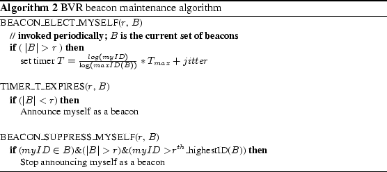
When the number of beacons alive falls below a configurable parameter
![]() , non-beacon nodes will nominate themselves as beacons. Using
ideas from SRM [5], each node sets a timer that is a function
of its unique identifier and, when the timer expires, it starts
acting like a beacon. If it detects that there are more than
, non-beacon nodes will nominate themselves as beacons. Using
ideas from SRM [5], each node sets a timer that is a function
of its unique identifier and, when the timer expires, it starts
acting like a beacon. If it detects that there are more than ![]() beacons with identifiers smaller than its identifier, it then ceases
to be a beacon. Algorithm 2 shows
our beacon selection algorithm. More sophisticated beacon
maintenance protocols can be designed to more fully optimize beacon
placement and suppression.
beacons with identifiers smaller than its identifier, it then ceases
to be a beacon. Algorithm 2 shows
our beacon selection algorithm. More sophisticated beacon
maintenance protocols can be designed to more fully optimize beacon
placement and suppression.
This soft-state based approach allows two mechanisms to recover from beacon failures. First, the hashing scheme allows the deterministic choice of backup beacons to replicate the information. The degree of replication depends on the expected failure rate of beacons. Second, the periodic updates will naturally populate a newly elected beacon that replaces a failed beacon. It is important to note that given the redundancy of the coordinate system, even slightly outdated information will lead the routes close to the destination. As we show in our experimental results, both the magnitude and the frequency of the changes to coordinates is small in practice.
To evaluate the BVR algorithm, we use extensive simulations and experiments on testbeds of real sensor motes. To aid the development of BVR and to better understand its behavior and design tradeoffs we start by evaluating BVR using a high-level simulator that abstracts away many of the vagaries of the underlying wireless medium. While clearly not representative of real radios, these simplifications allow us to explore questions of algorithm behavior over a wide range of network sizes, densities, and obstacles that would not be possible on a real testbed.
In practice however, the characteristics of wireless sensor networks impose a number of challenges on actual system development. For example, the mica2dot motes have severe resource constraints - just 4KB of RAM, typical packet payloads of 29 bytes etc. - and the wireless medium exhibits changing and imperfect connectivity. Hence, our next round of evaluation is at the actual implementation level. We present the implementation and experimental evaluation of our BVR prototype in Sections 5 and 6 respectively and our simulation results in this section.
Our simulator makes several simplifying assumptions. First, it
models nodes as having a fixed circular radio range; a node can
communicate with all and only those nodes that fall within its range.
Second, the simulator ignores the capacity of, and
congestion in, the network.
Finally, the simulator ignores packet losses.
While these assumptions are clearly unrealistic, they
allow the simulator to scale to tens of thousands of nodes.
We place nodes uniformly at random in a square
planar region, and we vary the total number of beacons ![]() , and the number
of routing beacons,
, and the number
of routing beacons, ![]() . In all our tests, we compare the results of routing
over BVR coordinates to greedy geographic routing over the true positions
of the nodes.
. In all our tests, we compare the results of routing
over BVR coordinates to greedy geographic routing over the true positions
of the nodes.
Our default simulation scenario uses a
3200 node network with nodes uniformly distributed in an
area of 200 ![]() 200 square units. The radio range is 8 units,
and average node degree is 16. Unless otherwise
stated, a node's neighbors are those nodes within
its one hop radius.
200 square units. The radio range is 8 units,
and average node degree is 16. Unless otherwise
stated, a node's neighbors are those nodes within
its one hop radius.
In our evaluation, we consider the following performance metrics:
(Greedy) success rate: The fraction of packets that are delivered to the destination without requiring flooding. We stress that the final scoped flooding phase ensures that all packets eventually reach their destination. This metric merely measures how often the scoped flooding is not required. Like previous virtual coordinate solutions [24,25], we report on the success of routing without scoped floods because that provides the most unambiguous evaluation of the quality of node coordinates themselves; e.g., scoped flooding, which will always succeed, does not depend on coordinates. If our results are comparable to those with true positions, then BVR would have overcome the need for geographic information in current proposals. Nonetheless, later in this section, we also present results on a metric we term transmission stretch that does explicitly account for the overhead of scoped floods.
Flood scope: The number of hops it takes to reach the destination in those cases when flooding is invoked.
Path stretch: The ratio of the path length of BVR to the path length of greedy routing using true positions.
Node load: The number of packets forwarded per node.
In each test, we're interested in understanding the overhead required to achieve good performance as measured by the above metrics. There are three main forms of overhead in BVR:
Control overhead: This is the total number of
flooding messages generated to compute and maintain node
coordinates and is directly dependent on ![]() , the total number of
beacons in the system. We measure control overhead in
terms of the total number of beacons that flood the
network. Ideally, we want to achieve high
performance with reasonably low
, the total number of
beacons in the system. We measure control overhead in
terms of the total number of beacons that flood the
network. Ideally, we want to achieve high
performance with reasonably low ![]() .
.
Per-packet header overhead: A destination is defined in
terms of its ![]() routing beacons. Because the destination
position is carried in the header of every packet for routing purposes,
routing beacons. Because the destination
position is carried in the header of every packet for routing purposes,
![]() should be reasonably low.
should be reasonably low.
Routing state: The number of neighbors a node maintains in its routing table.
![\includegraphics[width=7cm]{sylvia/routing_beacon_success}](img61.png) |
In this section, we consider the tradeoff between the routing success
rate and the flood scope on one hand, and the overhead due
to control traffic (![]() ) and per-packet state (
) and per-packet state (![]() ) on the
other hand.
We use our default simulation scenario and for each of ten repeated
experiments, we randomly choose
) on the
other hand.
We use our default simulation scenario and for each of ten repeated
experiments, we randomly choose ![]() beacons from the total
set of nodes. We vary
beacons from the total
set of nodes. We vary ![]() from
from ![]() to
to ![]() each time generating
each time generating
![]() routes between randomly selected pairs of nodes.
routes between randomly selected pairs of nodes.
Figure 1 plots the routing success rate
for an increasing total number of beacons (![]() ) at three
different values of
) at three
different values of ![]() , the number of routing beacons (
, the number of routing beacons (![]() ,
, ![]() , and
, and ![]() )
As expected, the success rate increases
with both the number of total beacons and the number of routing
beacons.
We draw a number of conclusions from these results.
We see that with just
)
As expected, the success rate increases
with both the number of total beacons and the number of routing
beacons.
We draw a number of conclusions from these results.
We see that with just ![]() routing beacons we can
achieve routing performance comparable to that using true positions.
The performance improvement in increasing
routing beacons we can
achieve routing performance comparable to that using true positions.
The performance improvement in increasing ![]() to 20
is marginal. Hence, from here on, we limit our tests to
using
to 20
is marginal. Hence, from here on, we limit our tests to
using ![]() routing beacons as a good compromise between
per-packet overhead and performance.
Using
routing beacons as a good compromise between
per-packet overhead and performance.
Using ![]() , we see that only between 20 to 30 total beacons (
, we see that only between 20 to 30 total beacons (![]() )
is sufficient to match the performance of true positions. At
less than 1% of the total number of nodes, this is very reasonable
flooding overhead. The scope of floods as a function of
)
is sufficient to match the performance of true positions. At
less than 1% of the total number of nodes, this is very reasonable
flooding overhead. The scope of floods as a function of ![]() decreases from 7 at
decreases from 7 at ![]() 10 to 3 at
10 to 3 at ![]() 70.
70.
The average path length in these tests was 17.5 hops and the path stretch, i.e., the length of the BVR path over the path length using greedy geographic routing over true positions, is 1.05. In all our tests, we found that the path stretch was always less than 1.1 and hence we don't present path stretch results from here on.
We also compared the distribution of the routing load over
nodes using BVR versus greedy geographic routing over
true positions and found that for most
nodes, the load is virtually identical though BVR does
impose slightly higher load on the nodes in the immediate vicinity
of beacons. For example, for the above test using ![]() and
and ![]() ,
the 90th percentile load per node was 48 messages using BVR compared to
37 messages using true positions.
,
the 90th percentile load per node was 48 messages using BVR compared to
37 messages using true positions.
In summary, we see that BVR can roughly match the performance of greedy geographic routing over true positions with a small number of beacons using only its one-hop neighbors.
![\includegraphics[width=7cm]{sylvia/density.eps}](img69.png) |
In this section, we consider the impact of the node density on the
routing success rate. Figure 2 plots the
success rate for the original density of ![]() nodes per communication
range, and for a lower density of
nodes per communication
range, and for a lower density of ![]() nodes per communication
range.
While at high density the performance of both approaches
is comparable, we see that at low densities BVR performs much better than greedy
geographic routing with true positions. In
particular, while the success rate of the greedy routing is about
nodes per communication
range.
While at high density the performance of both approaches
is comparable, we see that at low densities BVR performs much better than greedy
geographic routing with true positions. In
particular, while the success rate of the greedy routing is about
![]() , the success rate of BVR reaches
, the success rate of BVR reaches ![]() with
with ![]() beacons, and
beacons, and
![]() with
with ![]() beacons. Thus, BVR achieves an almost
beacons. Thus, BVR achieves an almost ![]() improvement in the success rate compared to greedy routing with true
positions. This is because the node coordinates in BVR are derived
from the connectivity information, and not from their geographic
positions which may be misleading in the presence of the voids
that occur at low densities.
improvement in the success rate compared to greedy routing with true
positions. This is because the node coordinates in BVR are derived
from the connectivity information, and not from their geographic
positions which may be misleading in the presence of the voids
that occur at low densities.
![\includegraphics[width=7cm]{sylvia/2-hop-on-demand-and-density}](img78.png) |
These results reflect the inherent tradeoff between the amount of routing state per node and the success rate of greedy routing. At lower densities, each node has fewer immediate neighbors and hence the performance of greedy routing drops. One possibility to improve the performance of our greedy routing is to have nodes maintain state for nodes beyond their one-hop neighborhood. This however increases the overhead and complexity of maintaining routing state. To retain high success rates without greatly (or needlessly) increasing the routing state per node, we propose the use of on-demand two-hop neighbor acquisition. Under this approach, a node starts out using only its immediate (one-hop) neighbors. If it cannot forward a message greedily, it fetches its immediate neighbors' neighbors and adds this two-hop neighbors to its routing table. The intuition behind this approach is that the number of local minima in a graph is far smaller than the total number of nodes. Thus, the on-demand approach to augmenting neighbor state allows only those nodes that require the additional state to incur the overhead of maintaining this state.
To evaluate the effectiveness of using on-demand two-hop neighbor
acquisition, we repeat the experiments in
Figure 2 using this approach. The results
are plotted in Figure 3. Not surprisingly, this
approach greatly improves the routing success rate. With only ![]() beacons, the success rate of BVR exceeds
beacons, the success rate of BVR exceeds ![]() for the high density
network, and
for the high density
network, and ![]() for the low density
network. Table 3 shows the average and
worst case increase in the per-node routing state for both BVR
and true positions. Using BVR, at high density, only
for the low density
network. Table 3 shows the average and
worst case increase in the per-node routing state for both BVR
and true positions. Using BVR, at high density, only ![]() of nodes
fetch their two-hop neighbors while
of nodes
fetch their two-hop neighbors while ![]() of nodes do so at the
lower densities. Thus acquiring two-hop neighbors on demand
represents a big win at a fairly low cost.
of nodes do so at the
lower densities. Thus acquiring two-hop neighbors on demand
represents a big win at a fairly low cost.
|
![\includegraphics[width=7cm]{sylvia/number_of_beacons.eps}](img84.png) |
In this section, we ask the following question: how many beacons are
needed to achieve a target success rate as the network size increases?
To answer this question, we set the target of the routing success rate
at ![]() . Figure 4 plots the number of
beacons required to achieve this target for both BVR using a one-hop
neighborhood, and BVR using on-demand two-hop neighbor acquisition. In
both cases the number of routing beacons is
. Figure 4 plots the number of
beacons required to achieve this target for both BVR using a one-hop
neighborhood, and BVR using on-demand two-hop neighbor acquisition. In
both cases the number of routing beacons is ![]() .
.
There are two points worth noting. First, the number of beacons for
the on-demand two-hop neighborhood remains constant at ![]() as the
network size increases from
as the
network size increases from ![]() to
to ![]() nodes. Second, while the
number of beacons in the case of BVR with one-hop neighborhood
increases as the network size increases, this number is still very
small. When the network is greater than
nodes. Second, while the
number of beacons in the case of BVR with one-hop neighborhood
increases as the network size increases, this number is still very
small. When the network is greater than ![]() nodes, the number of
beacons for the one-hop neighborhood never exceeds
nodes, the number of
beacons for the one-hop neighborhood never exceeds ![]() .
.
These results show that the number of beacons required to achieve low flooding rates grows slowly with the size of the system.
We now study the BVR performance in the presence of
obstacles. We model obstacles as horizontal or vertical ``walls'' with
lengths of ![]() or
or ![]() units. For comparison, recall that the radio
range of a node is 8 units.
units. For comparison, recall that the radio
range of a node is 8 units.
Table 4 shows the success rates of BVR routing over
a one-hop neighborhood for different numbers of obstacles. For each
entry, we also show, in parentheses, the success rate of greedy
routing using true positions. Surprisingly, as the number of
obstacles and/or their length increases, the decrease in success rate
using BVR is not significant. In the worst case the success
rate drops only from ![]() to
to ![]() . For comparison, the success
rate of greedy routing with true positions drops from
. For comparison, the success
rate of greedy routing with true positions drops from ![]() to
to
![]() ! Again, this is because the node coordinates in
BVR reflect their connectivity instead of their true positions.
! Again, this is because the node coordinates in
BVR reflect their connectivity instead of their true positions.
![\includegraphics[width=7cm]{sylvia/overhead_vs_beacons.eps}](img93.png) |
This section describes our prototype implementation
of BVR in TinyOS [11] for the mica2dot motes.
The resource constraints of the mote hardware and the vagaries
of the wireless medium lead to a number of practical difficulties
not addressed in our discussion so far.
In particular, the following are four key issues that must be addressed
in a real implementation:
Link estimation:
In a wireless medium, the notion of an individual link is
itself ill-defined as the quality
of communication varies dramatically across nodes, distance and time.
Link estimation is used to characterize a link as the probability of
successful communication rather than a simple binary on/off relation.
Link/neighbor selection: The limited memory in the mote
hardware prevents a node from holding state for all its links. Link selection
determines the set of neighbors in a node's routing table.
Distance estimation: Recall that our BVR algorithm defines a
node's coordinates as its distance in hops to a set of beacons. We
describe how we define the hop distance
from a node to a beacon when individual links are themselves defined in terms
of a quality estimate.
Route selection: This addresses how a node forwards packets in the face
of lossy links.
Each of the above is a research problem in itself (see [32,33] for a detailed exploration of some of these issues); while our implementation makes what we believe are sound choices for each, a comprehensive exploration of the design space for each individual component is beyond the scope of this paper. We describe our solutions to each of the above problems and present the results of our system evaluation in the following section.
Currently, our prototype sets the number of routing beacons equal
to the total number of beacons (![]() ) and does not implement
the successive dropping of beacons in computing distances for greedy forwarding
(i.e., a node that cannot make greedy progress
using all available beacons switches directly to fallback mode).
We also do not implement the on-demand
neighbor acquisition described in the previous section.
If anything, these simplifications can only degrade performance
relative to our earlier simulation results.
) and does not implement
the successive dropping of beacons in computing distances for greedy forwarding
(i.e., a node that cannot make greedy progress
using all available beacons switches directly to fallback mode).
We also do not implement the on-demand
neighbor acquisition described in the previous section.
If anything, these simplifications can only degrade performance
relative to our earlier simulation results.
We implemented a passive link estimator, based on the work by Woo et al.[32]. We tag all outgoing packets with a sequence number, such that the receiving nodes can estimate the fraction of packets that are lost from each source. We collect statistics in successive time windows, and the estimation is derived from an exponentially weighted moving average of the quality over time. This estimates the quality of incoming links. To accommodate link asymmetry, every node periodically transmits its current list of incoming link qualities. It is aided by the fact that nodes transmit at a minimum rate, making estimation more reliable: in BVR, nodes periodically broadcast ``hello'' messages used to announce coordinates and maintain the beacon trees. The link estimator is also responsible for detecting ``dead'' neighbors, and to keep a table with the best quality links.
Because motes have limited memory, a
node may not be able to (or may not want to devote the memory
needed to) hold state for all the nodes it might hear from.
Hence on the one hand we want a node to hold state for its highest
quality links but on the other hand the node does not have
the memory resources necessary to estimate the quality of all its links.
To tackle this problem we use a scheme that guarantees that a node's link
will store a set of neighbors with quality above a given low
quality replacement threshold ![]() .
When a node is first inserted in the link table it is subject to
a probation period.
We set the probation period to be such that the link estimator would have converged to within
10% of the stable quality of the link.
An entry in the link table cannot be replaced unless it is past
probation and has a link quality below the replacement threshold.
In our prototype, we use a link table size
.
When a node is first inserted in the link table it is subject to
a probation period.
We set the probation period to be such that the link estimator would have converged to within
10% of the stable quality of the link.
An entry in the link table cannot be replaced unless it is past
probation and has a link quality below the replacement threshold.
In our prototype, we use a link table size ![]() of 18
neighbors, and set
of 18
neighbors, and set ![]() to 20%.
to 20%.
Central to BVR is a node's distance in hops to each beacon.
In the presence of lossy links, it is important to avoid using long and
unreliable links, which can give the false impression
of a low hopcount to the root. To this effect, nodes determine their
distance from the beacon by choosing parents that minimize the expected number
of transmissions (ETX) to the root [32] along the reverse path.
The ETX for one link with forward and reverse
transmission success probability ![]() and
and ![]() is
is
![]() , and
the ETX to the root is obtained incrementally by adding the ETX for each link.
A node's distance is the number of hops along such path. We use some hysteresis
when selecting parents with different hopcounts to increase the stability of the coordinates.
, and
the ETX to the root is obtained incrementally by adding the ETX for each link.
A node's distance is the number of hops along such path. We use some hysteresis
when selecting parents with different hopcounts to increase the stability of the coordinates.
When selecting the next hop in forwarding a message,
our BVR prototype takes into account both the progress in the distance
function and the quality of the links. Usually, the nodes
that make the most progress are also further away, and present
poor link quality. We order all links that make some progress
towards the destination by expected progress: the product of the bidirectional link
quality and the actual progress in the distance function. This is analogous to the
![]() metric from [28],
found to be optimal for geographic routing. When sending a message, we use two optimizations for reliability.
First, we use link level acknowledgments with up to
five retransmissions. Second, if a transmissions fails despite the multiple
retries, the node will try the other neighbors in decreasing order
of their expected progress. Only when it has exhausted all possible next hop options will the
node revert to fallback mode.
metric from [28],
found to be optimal for geographic routing. When sending a message, we use two optimizations for reliability.
First, we use link level acknowledgments with up to
five retransmissions. Second, if a transmissions fails despite the multiple
retries, the node will try the other neighbors in decreasing order
of their expected progress. Only when it has exhausted all possible next hop options will the
node revert to fallback mode.
Table 5 summarizes our various parameter settings. We selected these based on both our own experience and those reported by Woo et al.[32] with the mote radios. We intend to achieve good tradeoff between maintaining freshness of the routing state, and the amount of control traffic generated. A back-of-the-envelope calculation based on our measured channel capacity indicates that our timer settings lead to control traffic of approximately 5% of the channel capacity. Fully understanding the generality of our parameter selection is beyond the scope of this paper and a topic we intend to explore. Nonetheless, because sensornet topologies (unlike most other networks) are dependent on so many deployment specific issues -- interference and obstacles in the physical environment, number and layout of nodes, power settings, etc. -- we do expect deployments to always involve some amount of a priori calibration to guide parameter selection.
![\includegraphics[width=7cm]{figures/testbed-neighborhood-map.soda.eps}](img102.png)
|
On both testbeds, we set parameters as described in the previous section. Our experiments consist of a setup phase of several minutes to allow the link estimations to converge, beacon trees to be constructed and nodes to discover their neighbors' positions. After this setup phase, we issue route commands from a PC to individual motes over the Ethernet backchannel.
In the reminder of this section we evaluate four main aspects of the
BVR design:
Link Estimation: We validate that a node indeed selects high quality
neighbors. This is important because, as has been reported, the details
of link estimation are at once tricky and greatly impact performance.
Moreover, because link quality is a function of environment, topology and traffic
patterns, we could not just expect behavior identical to previous
studies [32,33].
Routing Performance: We evaluate BVR's success rate on
two testbeds under increasing load. We find that the routing
success rate is high (over 97%) when the network load is low, and
degrades gracefully as the load increases.
Dynamics: We evaluate performance under
both node and beacon failures and show that BVR sustains high
performance even under high node failure rate.
Coordinate Stability: Because many applications may use node
coordinates as addresses, it is important that these
coordinates vary little in magnitude and over time. We find
that BVR coordinates are quite stable.
We also examined the network-wide connectivity in our testbeds. Figure 6 shows a snapshot of the network, drawn to scale, and the connectivity as determined by the neighbor tables at each mote on the 74 node Univ-Net testbed. We see that network connectivity is frequently not congruent with physical distance (e.g., mote pairs 32-30, 32-9, 26-37, 35-27, 54-59). We also note the existence of short but asymmetric links (motes 24-26).
For the same testbed, Figure 8 shows the relation between link quality and physical distance between pairs of nodes that are neighbors (as determined by BVR's link and neighbor selection algorithms). While BVR select predominantly high quality neighbors, these are quite frequently not physically close; in fact, a fair number of neighbors are more than halfway across the network. Note that these observations contradict the circular radio assumptions made by typical geographic routing algorithms and lend credibility to the need for connectivity-derived coordinates.
![\includegraphics[width=7cm]{figures/combined.qualities.hist.box.eps}](img103.png)
|
![\includegraphics[width=7cm]{figures/soda_large_kill.10.14.gz.quality_vs_distance.eps}](img104.png)
|
![\includegraphics[width=7cm]{figures/log.200503292322.routes.route_histogram.100.eps}](img105.png)
![\includegraphics[width=7cm]{figures/soda.large_test.8beacons.thoughtput_test.eps}](img106.png)
|
Figure 9 present results for the Office-Net and Univ-Net testbeds. The graphs show: (1) the overall success rate measured as the fraction of routes that arrived at the target destination, (2) the fraction of routes that required scoped flooding, (3) the fraction of routes that failed due to contention drops where contention drops are packets that were dropped due to a lack of sending buffers along the internal send path in the mote network stack and (4) failures which are routes that failed despite the multiple retries; i.e., the message was repeatedly sent out over the channel but no acknowledgments were received. The graph also plots the aggregate network route request rate over time with the scale on the right hand Y axis. Our tests start (after the setup phase) with a rate of one route request per second for a period of approximately one hour; after this we increase the route request rate every 400 seconds up to a maximum rate of approximately 8 routes/second.
On Office-Net, BVR achieved an average success rate (greedy or flood) of 99.9% until a load of about 8.8 requests/second, at which point we start seeing a small number of contention drops. 1.2% of all route requests in this period resulted in scoped flooding (with an average scope of 2 hops), and less than 0.1% were contention drops. Similarly for Univ-Net, the average success rate was 98.5%. 5.5% of all routes required scoped flooding (with again an average scope of 2 hops), there were no contention drops, and 1.15% of routes failed due to persistent loss. We repeated the above tests with a larger number of beacons and recorded similarly high success rates; due to space considerations, we do not present these here. These experiments indicate that our BVR implementation works correctly in a real deployment, and can sustain a significant workload of routing messages.
Sensor nodes are vulnerable to temporary or permanent failures due to depleted energy resources, or damage from weather conditions. We test BVR's resilience to such failures using both TOSSIM and real testbed experimentation. We show that BVR can recover from both node and beacon failures and sustain good routing performance without incurring high overhead. We first evaluate BVR's robustness to non-beacon node failure using the Office-Net testbed and then evaluate robustness to beacon failure in TOSSIM.
![\includegraphics[width=7cm]{figures/log.200503290209.routes.route_histogram.100.eps}](img107.png)
|
Section 3 discussed the need to maintain a reasonable number of beacon nodes in the network. Our BVR implementation includes Algorithm 2 which we tested using TOSSIM. Our TOSSIM experiments choose a baseline configuration of 100 motes with 8 beacons and expected node degree of 12. We use TOSSIM's lossy link generator, which is itself based on empirical data and includes lossy and asymmetric connectivity. After a 30 minute setup phase, we initiate a constant rate of one route per second between random node pairs and kill a randomly selected beacon node at increasing rates. Success rates are computed in 100 second time windows under traffic load of 1 route request per second.
Figure 11 shows a typical simulation run. We see that routing performance does not degrade with occasional beacon failures, and tolerates high failure rates reasonably well. This is largely because BVR routes well with even a partial beacon vector set. Residual beacon vectors from recently deceased beacons also serve as hints for packet forwarding. Closer examination of the test log shows that the convergence time of the beacon replenishment is fast, and dependent as expected on the network diameter and frequency of neighbor exchanges. Candidate beacons are efficiently suppressed and hence we observed no significant communication overhead.
![\includegraphics[width=0.95\textwidth]{figures/log.200503292322.sorted.e6000.motes_w_changes_vs_time.100.eps}](img108.png)
|
![\includegraphics[width=0.95\textwidth]{figures/log.200503292322.sorted.e6000.motes_w_changes_vs_time.100.eps}](img109.png)
|
![\includegraphics[width=0.95\textwidth]{figures/combined_mag_changes_new_small_intel.eps}](img110.png)
|
In Figure 12 we look at the number of nodes with changes in coordinates per fixed 100-second intervals for a run in Office-Net, with a load of one route per second. This approximates the minimum aggregate update traffic that would be seen in the network if motes were to update at most once every such period, when their coordinates changed. From the graph we see that there are more nodes with changes in the beginning, as the link estimators are stabilizing, and then there is a reduction. The average number of motes with changes per slot is 0.95, and the 95th percentile is 9. We also looked at 10 second intervals, and the average number of motes with changes is 0.13 per interval, which is relatively consistent. In terms of number of changes, during this period of 100 minutes, 90% of the motes had 5 or fewer changes in coordinates. The results we saw in the Univ-Net testbed are similar. Figure 13 plots the distribution of the magnitude of individual coordinate changes over all coordinate changes. Magnitude here is simply the change in a node's distance to a beacon; i.e., a change in distance to a beacon from 5 hops to 3 hops would be counted as a magnitude of 2. We see that change, when it occurs, is small: for both testbeds, in this case, at least 80% of the changes were of 2 or less hops. These results suggest that BVR can be used as a stable routing solution that is scalable, robust, and does not unduly load beacons.
However, we are at the very early stages of our investigation. We need to better understand how BVR's performance is linked to radio stability, the generality of our parameter selection as well as more rigorous approaches to tuning these parameters. Most importantly however, we have not yet implemented any applications on top of BVR, so we don't yet know if it provides a suitably stable substrate on which to build. All of these items represent future work.
|
This paper was originally published in the
Proceedings of the 2nd Symposium on Networked Systems Design and Implementation,
May 2–4, 2005, Boston, MA, USA Last changed: 2 May 2005 aw |
|
![\begin{algorithm}
% latex2html id marker 371\caption{BVR forwarding algorithm}...
...pe ${P}.\mathcal{P}{(dst)}[fallback\_bcn]$
\par
\end{algorithmic}\end{algorithm}](img51.png)