| From | T | U | V | T+U+V | Adjusted |
|---|---|---|---|---|---|
| AP | 97.85 | 96.88 | 96.14 | 98.53 | 98.53 |
| 97.48 | 93.65 | 92.92 | 97.72 | 97.72 | |
| 61.09 | 88.51 | 88.67 | 88.96 | 93.31 | |
| Total | 88.92 | 93.91 | 93.40 | 95.74 | 96.97 |
Table 2 analyzes the sequence numbers for
the same controlled experiments as represented in
Table 1. As MAC sequence numbers are generated
per device, we examined the MAC sequence numbers of the AP, client
![]() and client
and client ![]() separately. Table 2
shows that as data from sniffers
separately. Table 2
shows that as data from sniffers ![]() ,
, ![]() , and
, and ![]() are merged, the
capture performance for AP,
are merged, the
capture performance for AP, ![]() and
and ![]() increases to 98.5%,
97.7%, and 89% respectively (with a further increase to 93%
in the discussion below). The numbers in the table reflect the
gap between different frames captured by the sniffers.
increases to 98.5%,
97.7%, and 89% respectively (with a further increase to 93%
in the discussion below). The numbers in the table reflect the
gap between different frames captured by the sniffers.
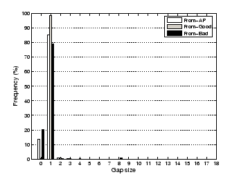
Figure 3 shows histograms of the gap size between
two consecutive frames for the case of using the three sniffers.
Note that a gap of zero means that a frame has been retransmitted,
while a gap of 1 means that there are no missing frames between
these two frames. To calculate the number of missing frames, we
count the gaps of greater than 1. Let ![]() denote the number
of occurrences of gap size
denote the number
of occurrences of gap size ![]() in Figure 3.
Then, we can calculate the number of missing frames (
in Figure 3.
Then, we can calculate the number of missing frames (![]() )
by
)
by
![]() . The column labeled
`T+U+V' in Table 2 can be obtained by
. The column labeled
`T+U+V' in Table 2 can be obtained by
![]() ,
where
,
where ![]() denotes the number of distinct captured frames.
denotes the number of distinct captured frames.
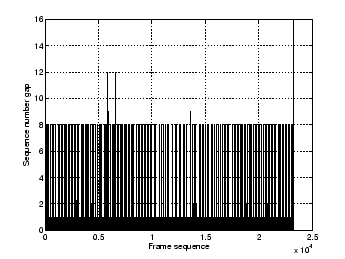
Figure 4 takes a closer look at the Bad client case. The x-axis represents the received frame sequence number and the y-axis represents the gap before this frame. There was a periodic gap of 8, i.e., a measurement loss of 7 frames. By looking into the traces we found that these periodic behavior was due to the Bad client performing periodic active scanning searching for better APs. Since this process involves sending probe request frames on different channels 13 (13), the sequence numbers were not captured by our sniffers, which sniffed the traffic on only one channel. If these missed probe request frames are added to the loss statistics in Table 2, the capture accuracy for the Bad client increases to 93.31% and the overall capture performance increases to 96.97% (as shown in the Adjusted column in Table 2). This means that the WM statistics differ by at most 3.03% from the actual statistics.