| ||||||||||||||||||||||||||||||||||||||||||||||||||||
|
MobiSys '05 Paper
[MobiSys '05 Technical Program]
The Horus WLAN Location Determination System Moustafa Youssef and Ashok Agrawala
AbstractWe present the design and implementation of the Horus WLAN location determination system. The design of the Horus system aims at satisfying two goals: high accuracy and low computational requirements. The Horus system identifies different causes for the wireless channel variations and addresses them to achieve its high accuracy. It uses location-clustering techniques to reduce the computational requirements of the algorithm. The lightweight Horus algorithm helps in supporting a larger number of users by running the algorithm at the clients.We discuss the different components of the Horus system and its implementation under two different operating systems and evaluate the performance of the Horus system on two testbeds. Our results show that the Horus system achieves its goal. It has an error of less than 0.6 meter on the average and its computational requirements are more than an order of magnitude better than other WLAN location determination systems. Moreover, the techniques developed in the context of the Horus system are general and can be applied to other WLAN location determination systems to enhance their accuracy. We also report lessons learned from experimenting with the Horus system and provide directions for future work.
1 IntroductionHorus is an RF-based location determination system. It is currently implemented in the context of 802.11 wireless LANs [25]. The system uses the signal strength observed for frames transmitted by the access points to infer the user location. Since the wireless cards measure the signal strength information of the received frames as part of their normal operation, this makes the Horus system a software solution on top of the wireless network infrastructure. There are two classes of WLAN location determination systems: client-based and infrastructure-based. Both have their own set of applications. Horus is currently implemented as a client-based system. A large class of applications [10], including location-sensitive content delivery, direction finding, asset tracking, and emergency notification, can be built on top of the Horus system.WLAN location determination is an active research area [33,30,34,31,29,5,6,22,8,9,21,20,17,13,15,12]. WLAN location determination systems usually work in two phases: an offline training phase and an online location determination phase. During the offline phase, the system tabulates the signal strength received from the access points at selected locations in the area of interest, resulting in a so-called radio map . During the location determination phase, the system use the signal strength samples received from the access points to ``search'' the radio map to estimate the user location. Radio-map based techniques can be categorized into two broad categories: deterministic techniques and probabilistic techniques. Deterministic techniques [5,6,22] represent the signal strength of an access point at a location by a scalar value, for example, the mean value, and use non-probabilistic approaches to estimate the user location. For example, in the Radar system [5,6] the authors use nearest neighborhood techniques to infer the user location. On the other hand, probabilistic techniques [33,30,34,29,31,8,9,21,20,17,13] store information about the signal strength distributions from the access points in the radio map and use probabilistic techniques to estimate the user location. For example, the Nibble system [8,9 ] uses a Bayesian Network approach to estimate the user location. The Horus system lies in the probabilistic techniques category. The design of the Horus system aims at satisfying two goals: high accuracy and low computational requirements. The Horus system identifies different causes for the wireless channel variations and addresses them to achieve its high accuracy. It uses location-clustering techniques to reduce the computational requirements of the algorithm. The lightweight Horus algorithm allows it to be implemented in energy-constrained devices. This non-centralized implementation helps in supporting a larger number of users. In this paper, we present the different components of the Horus system and show how they work together to achieve its goals. We discuss our Horus implementation under two different operating systems and evaluate its performance on two different indoor testbeds. The rest of the paper is structured as follows: in the next section, we describe the different causes of variations in the wireless channel. In Section 3 we present the different components of the Horus system that deal with the noisy characteristics of the wireless channel. We present the results of testing the Horus system on two different testbeds in Section 4. Section 5 presents our experience while building the Horus system. In Section 6 we discuss related work. Finally, Section 7 concludes the paper and provides directions for future work.
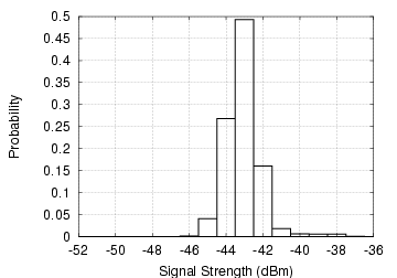
In this section, we identify the different causes of variations in the wireless
channel quality and how they affect the WLAN location determination systems. We
are mainly concerned with the variations that affect the received signal
strength. We start by describing our sampling process. Then, we categorize the
variations in the wireless channel as temporal variations and spatial
variations. We performed all the experiments in this section in a typical
office building, measured during the day when people are around.
| |||||||||||||||||||||||||||||||||||||||||||||||||||||||||||||||||||||||||||
|
|
Large-scale variations are desirable in RF-based systems as they lead to changing the signature stored in the radio map for different locations and, hence, better differentiation between these locations.
Dealing with small-scale variations is challenging. To limit the radio map size and the time required to build the radio map, selected radio map locations are typically placed more than a meter apart. This means that the radio map does not capture small-scale variations leading to decreased accuracy in the current WLAN location systems.
In the next section, we indicate how the Horus system handles these temporal and spacial variations.
|
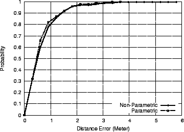
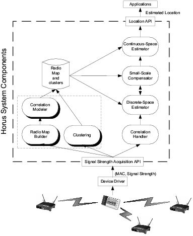
The radio map stores the distribution of signal strength received from each access point at each sampled location. There are two modes for operation of the Horus system: one uses non-parametric distributions and the other uses parametric distributions.
The Clustering module is used to group radio map locations based on the access points covering them. Clustering is used to reduce the computational requirements of the system and, hence, conserve power (Section 3.7 ).
The Discrete Space Estimator module returns the radio map location that has the maximum probability given the received signal strength vector from different access points (Section 3.3 ).
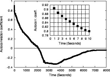
The Correlation Modelling and Handling modules use an autoregressive
model to capture the correlation between consecutive samples from the same
access point. This model is used to obtain a better discrete location estimate
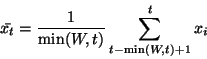
using the average of ![]() correlated samples (Section 3.4
).
correlated samples (Section 3.4
).
The Continuous Space Estimator takes as an input the discrete estimated user location, one of the radio map locations, and returns a more accurate estimate of the user location in the continuous space (Section 3.5 ).
The Small-Scale Compensator module handles the small-scale variation characteristics of the wireless channel (Section 3.6 ).
We start by laying out the mathematical framework for the approach then give details about different components of the system.
|
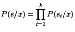
The problem becomes, given a signal strength vector
![]() , we want to find the location
, we want to find the location
![]() that maximizes the probability
that maximizes the probability ![]() .
.
In the next section, we assume a discrete
![]() space. We discuss the continuous space case in Section 3.5.
space. We discuss the continuous space case in Section 3.5.
The signal-strength histogram can be approximated by a parametric distribution such as the Gaussian distribution. We compare the performance of the discrete-space estimator based on the parametric and non-parametric distributions in the Section 4 .
Let ![]() be the stationary time series representing the samples from an access
point, where
be the stationary time series representing the samples from an access
point, where ![]() is the discrete time index.
is the discrete time index. ![]() can be represented as a first order autoregressive model [7
] as:
can be represented as a first order autoregressive model [7
] as:
where ![]() is a noise process, independent of
is a noise process, independent of ![]() ,
and
,
and ![]() is a parameter that determines the degree of autocorrelation of the original
samples. Moreover, different samples from
is a parameter that determines the degree of autocorrelation of the original
samples. Moreover, different samples from ![]() are independent and identically distributed (i.i.d.).
are independent and identically distributed (i.i.d.).
The model in Equation 4 states
that the current signal strength value (![]() )
is a linear aggregate of the previous signal strength value (
)
is a linear aggregate of the previous signal strength value (![]() )
and an independent noise value (
)
and an independent noise value (![]() ).
The parameter
).
The parameter ![]() gives flexibility to the model as it can be used to determine the degree of
autocorrelation of the original process. For example, if
gives flexibility to the model as it can be used to determine the degree of
autocorrelation of the original process. For example, if ![]() is zero, the samples of the process
is zero, the samples of the process ![]() are i.i.d.'s, whereas if
are i.i.d.'s, whereas if ![]() is 1 the original samples are identical (autocorrelation=1).
is 1 the original samples are identical (autocorrelation=1).
Assuming that the signal strength distribution of samples from an access point
is Gaussian with mean ![]() and variance
and variance ![]() ,
we have shown in [29,31]
that the distribution of the average of
,
we have shown in [29,31]
that the distribution of the average of ![]() correlated samples is a Gaussian distribution with mean
correlated samples is a Gaussian distribution with mean ![]() and variance given by:
and variance given by:
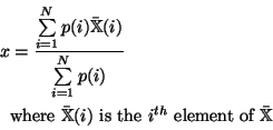
More formally, let ![]() be the probability of a location
be the probability of a location
![]() ,
i.e., the radio map, and let
,
i.e., the radio map, and let
![]() be the list of locations in the radio map ordered in a descending order
according to the normalized probability (the location with lower ID comes first
for locations with equal probability). The center of mass technique estimates
the current location
be the list of locations in the radio map ordered in a descending order
according to the normalized probability (the location with lower ID comes first
for locations with equal probability). The center of mass technique estimates
the current location ![]() as:
as:
More formally, given a stream of location estimates
![]() , the technique estimates the current location
, the technique estimates the current location ![]() at time
at time ![]() as:
as:
We compare the two techniques in Section 4.
The IT approach is based on the idea that each access point defines a subset of the radio map locations that are covered by this access point. These locations can be viewed as a cluster of locations whose key is the access point covering the locations in this cluster. If during the location determination phase we use the access points incrementally, one after the other, then starting with the first access point, we restrict our search space to the locations covered by this access point. The second access point chooses only the locations in the range of the first access point and covered by the second access point and so on, leading to a multi-level clustering process.
Notice that no preprocessing is required in the offline training phase. During
the online phase, a location ![]() belongs to a cluster whose key is access point
belongs to a cluster whose key is access point ![]() if there is information about access point
if there is information about access point ![]() at location
at location ![]() in the radio map.
in the radio map.
The algorithm works as follows. Given a sequence of observations from each access point, we start by sorting the access points in descending order according to the average received signal strength. For the first access point, the one with the strongest average signal strength, we calculate the probability of each location in the radio map set given the observation sequence from this access point alone. This gives us a set of candidate locations (locations that have non-zero probability). If the probability of the most probable location is ``significantly'' higher (according to a threshold) than the probability of the second most probable location, we return that most probable location as our location estimate, after consulting only one access point. If this is not the case, we go to the next access point in the sorted access point list. For this access point, we repeat the same process again, but only for the set of candidate locations obtained from the first access point. We study the performance of the IT approach in Section 4.
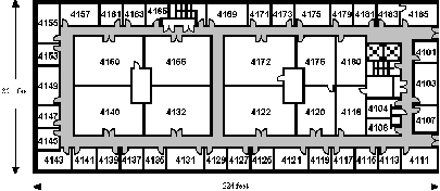
The radio map has 110 locations along the corridors and 62 locations inside the rooms. On the average, each location is covered by 6 access points. The Horus system was running under the Windows XP professional operating system.
|
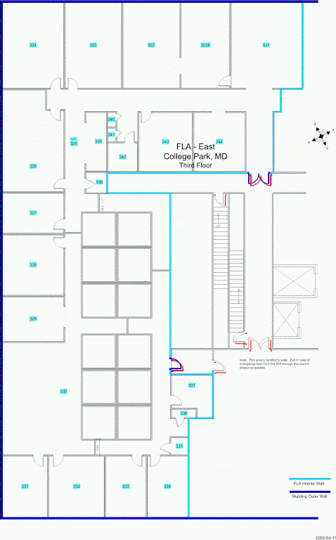
We have a total of 110 locations in the radio map. On the average, each location is covered by 4 access points. The Horus system was running under the Linux (kernel 2.5.7) operating system.
|
The training data was placed 1.52 meters (5 feet) apart for the first testbed and 2.13 meters apart for the second testbed (7 feet).
For each testbed, we selected 100 test locations to random cover the entire test area (none of them coincide with a training point). For both testbeds, the test set was collected by different persons on different days and times of day than the training set. This difference presents a realistic testbed and should, if anything, decrease the measured accuracy of our approach because it lessens the likelihood that the test data is a close match to the training data.
Table 1 shows the summary of the results for the two testbeds. Details for the second testbed can be found in [28 ].
Using the modified technique, the system average accuracy is enhanced by more than 19% using five signal-strength samples.

|
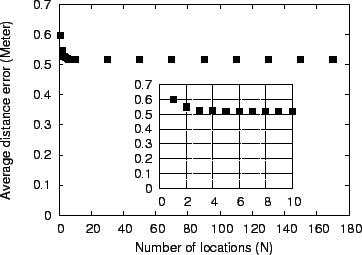
Center of Mass Technique: Figure 11
shows the effect of increasing the parameter ![]() (number of locations to interpolate between) on the performance of the center
of mass technique for the first testbed. Note that the special case of
(number of locations to interpolate between) on the performance of the center
of mass technique for the first testbed. Note that the special case of ![]() is equivalent to the discrete-space estimator output. The figures show that the
performance of the Horus system is enhanced by more than 13% for
is equivalent to the discrete-space estimator output. The figures show that the
performance of the Horus system is enhanced by more than 13% for ![]() .
.
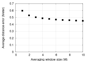
Time-averaging Technique: Figure 12
shows the effect of increasing the parameter ![]() (size of the averaging window) on the performance of the time-averaging
technique. The figures show that the larger the averaging window, the better
the accuracy. The performance of the Horus system is enhanced by more
than 24% for
(size of the averaging window) on the performance of the time-averaging
technique. The figures show that the larger the averaging window, the better
the accuracy. The performance of the Horus system is enhanced by more
than 24% for ![]() .
.
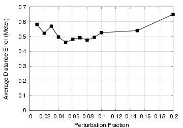
Figure 13 shows the effect of
changing the perturbation fraction (![]() , which is the amount by which to perturb each access point) on average error.
We can see from this figure that the best value for the perturbation fraction
is 0.05 for the first testbed. We use these values for the rest of this
section.
, which is the amount by which to perturb each access point) on average error.
We can see from this figure that the best value for the perturbation fraction
is 0.05 for the first testbed. We use these values for the rest of this
section.
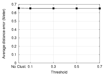
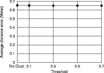
Figure 14 shows the effect of increasing the number of perturbed access points on the average distance error. The access points chosen at a location are the strongest access points in the set of access points that cover that location. The figure shows that perturbation technique is not sensitive to the number of access points. This means that perturbing one access point only is sufficient to enhance the performance.
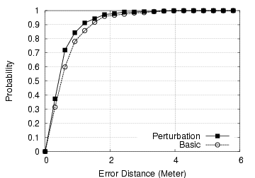
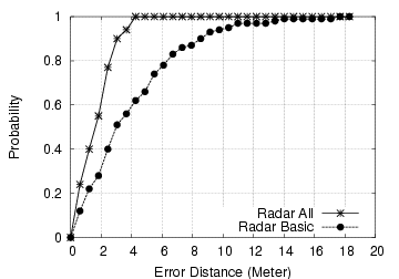
Figures 15 shows the effect of using the perturbation technique on the basic Horus system. The perturbation technique reduces the average distance error by more than 25% and the worst-case error is reduced by more than 30%.
![Effect of the parameter Threshold on the average number of operations per location estimate for the first testbed. The sub-figure shows the same curve for Threshold=[0.1,0.7].](img67.png)
|
Figures 18 shows the comparison for the two testbeds (the curve for the Radar system is truncated). Tables 3 summarizes the results. The table shows that the average accuracy of the Horus system is better than the Radar system by more than 89% for the first testbed and 82% for the second testbed. The worst case error is decreased by more than 93% for the first testbed and 70% for the second testbed.
[First testbed]
 [Second testbed]
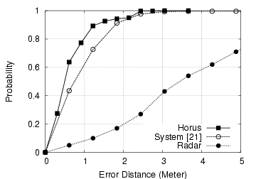
|
Comparing the probabilistic system in [21] to the Horus system shows that the average error is decreased by more than 35% for the first testbed and 27% for the second testbed. The worst case error is decreased by more than 78% for the first testbed and 70% for the second testbed. These results show the effectiveness of the proposed techniques.
The performance of the three systems is better in the first testbed than the
second testbed as the first testbed has a higher density of APs per location
and the calibration points were closer for the first testbed.
| Testbed 1 | Testbed 2 | |||||||||
| Median | Avg | Stdev | 90% | Max | Median | Avg | Stdev | 90% | Max | |
| Horus | 39 | 42 | 28 | 86 | 121 | 51 | 64 | 53 | 132 | 289 |
|---|---|---|---|---|---|---|---|---|---|---|
| System [21] | 48 | 65 | 63 | 143 | 578 | 72 | 86 | 77 | 181 | 991 |
| Radar | 296 | 400 | 326 | 853 | 1757 | 341 | 361 | 184 | 611 | 967 |
| Radar with Horus tech. | 161 | 193 | 107 | 302 | 423 | 142 | 195 | 106 | 332 | 483 |
Moreover, the Horus system leads to more than an order of magnitude savings in the number of multiplications required per location estimate compared to the other systems (250 multiplications for Horus compared to 2708 for the other two systems).
We also applied the enhancement discussed in this paper (without correlation handling) to the Radar system. We summarize the results is Table 3. These results show the effectiveness of the techniques proposed in the paper and that these techniques are general and can be applied to other WLAN location determination systems to enhance their accuracy.
Latency can be reduced by presenting the location estimate incrementally using
one sample at a time. The system need not to wait until it acquires the ![]() samples all at once. Instead, it can give a more accurate estimate of the
location as more samples become available by reporting the estimated location
given the partial samples it has. Other factors that affect the choice of the
value of
samples all at once. Instead, it can give a more accurate estimate of the
location as more samples become available by reporting the estimated location
given the partial samples it has. Other factors that affect the choice of the
value of ![]() are the user mobility rate and the sampling rate. The higher the user mobility
rate or the sampling rate, the lower the value of
are the user mobility rate and the sampling rate. The higher the user mobility
rate or the sampling rate, the lower the value of ![]() .
.
Our experience with the Horus system shows that the Laptop or PDA used for the calibration has no effect on the accuracy if a different device is used in tracking. APs from different manufacturers can be used without affecting the accuracy since the radio map captures the signature of the AP at each location (note that the second testbed uses mixed types of APs). The 802.11h specifications, however, require APs to have transmission power control (TPC) and dynamic frequency selection (DFS). This presents an open research direction for the current WLAN location determination systems as they assume that the AP transmission power does not change over time.
The main factor that may affect the accuracy when changing hardware is the wireless card. Our experience shows that cards from the same manufacture are inter-changeable. The good news is that a linear mapping exists between different NICs [13]. Unfortunately, some of the cards in the market are so noisy [27 ] that with this linear mapping the obtained radio map is not representative of the environment. We found that Orinoco cards and Cisco cards are stable, in terms of signal-strength measurements.
Our experience with both systems shows that drivers under Linux conform to the Wireless Extensions APIs better than Windows Drivers do with the NDIS. For example, under the Windows, some cards, like the Cisco card, respond to scans with low frequency (every 2-3 seconds) and return only one AP. We hope that future versions of the driver will have better support for the NDIS interface. Moreover for both systems, better active scanning techniques needs to be developed to reduce the scanning overhead.
Compared with these systems, WLAN location determination systems are software based (do not require specialized hardware) and may provide more ubiquitous coverage. This feature adds to the value of the wireless data network.
The Daedalus project [14 ] developed a system for coarse-grained user location. A mobile host estimates its location to be the same as the base station to which it is attached. Therefore, the accuracy of the system is limited by the access point density.
The RADAR system [5 ] uses the RF signal strength as an indication of the distance between the transmitter and receiver. During an offline phase, the system builds a radio map for the RF signal strength from a fixed number of receivers. During normal operation, the RF signal strength of the mobile client is measured by a set of fixed receivers and is sent to a central controller. The central controller uses a K-nearest approach to determine the location from the radio map that best fits the collected signal strength information.
The Aura system proposed in [22 ] uses two techniques: pattern matching (PM) and triangulation, mapping and interpolation (TMI). The PM approach is very similar to the RADAR approach. In the TMI technique, the physical position of all the access points in the area needs to be known and a function is required to map signal strength onto distances. They generate a set of training points at each trained position. The interpolation of the training data allows the algorithm to use less training data than the PM approach. During the online phase, they use the approximate function they got from the training data to generate contours and they calculate the intersection between different contours yielding the signal space position of the user. The nearest set of mappings from the signal-space to the physical space is found by applying a weighted average, based on proximity, to the signal space position.
The Nibble location system, from UCLA, uses a Bayesian network to infer a user location [8 ]. Their Bayesian network model include nodes for location, noise, and access points (sensors). The signal to noise ratio observed from an access point at a given location is taken as an indication of that location. The system also quantizes the SNR into four levels: high, medium, low, and none. The system stores the joint distribution between all the random variables of the system.
Another system, [21], uses Bayesian inversion to return the location that maximizes the probability of the received signal strength vector. The system stores the signal strength histograms in the radio map and uses them in the online phase to estimate the user location. Yet, another system, [17 ], applies the same technique to the robotics domain.
The Horus system is unique in defining the possible causes of variations in the received signal strength vector and devising techniques to overcome them, namely providing the correlation modeler, correlation handler, continuous space estimator, and small-space compensator modules. Moreover, it reduces the computational requirements of the location determination algorithm by applying location-clustering techniques. This allows the Horus system to achieve its goals of high accuracy and low energy consumption.
The Horus system models the signal strength distributions received from access points using parametric and non-parametric distributions. By exploiting the distributions, the Horus system reduces the effect of temporal variations.
We showed that the correlation of the samples from the same access point can be as high as 0.9. Experiments showed that under the independence assumption, as the number of averaged samples increases, the performance degrades. Therefore, we introduced the correlation modeler and handling modules that use an autoregressive model for handling the correlation between samples from the same access point. Using the modified technique, the system average accuracy is enhanced by more than 19% for the first testbed and 11% for the second testbed.
The Horus system uses the Perturbation technique for handling small-scale variations. The perturbation technique enhances the average distance error by more than 25% for the first testbed and more than 21% for the second testbed. Moreover, the worst-case error is reduced by more than 30% for the two testbeds.
The basic Horus technique chooses the estimated location from the discrete set of radio map locations. We described two techniques for allowing continuous-space estimation: the Center of Mass technique and the Time-Averaging technique. Using the Center of Mass technique, the accuracy of the Horus system was increased by more than 13% for the first testbed and by more than 6% for the second testbed compared to the basic technique. The Time-Averaging technique enhances the performance of the Horus system by more than 24% for the first testbed and more than 15% for the second testbed. The two techniques are independent and can be applied together.
We also compared the performance of the Horus system to the performance of the Radar system. We showed that the average accuracy of the Horus system is better than the Radar system by more than 89% for the first testbed and 82% for the second testbed. The worst case error is decreased by more than 93% for the first testbed and 70% for the second testbed. Comparing the probabilistic system in [21] to the Horus system shows that the average error is decreased by more than 35% for the first testbed and 27% for the second testbed. The worst case error is decreased by more than 78% for the first testbed and 70% for the second testbed. These results show the effectiveness of the proposed techniques. In terms of computational requirements, the Horus system is more efficient by more than an order of magnitude.
The proposed modules are all applicable to any of the current WLAN location determination systems. We show the result of applying the techniques of the Horus system to the Radar system. The results show that the average distance error is reduced by more than 58% for the first testbed and by more than 54% for the second testbed. The worst case error is decreased by more than 76% for the first testbed and by more than 48% for the second testbed.
As part of our ongoing work we are experimenting with different clustering techniques. Automating the radio-map generation process is a possible research area. The Horus system provides an API for location-aware applications and services. We are looking at designing and developing applications and services over the Horus system. A possible future extension is to dynamically change the system parameters based on the environment, such as changing the averaging window size as the user speed changes or using a time-dependent radio map. We are also working on the theoretical analysis of different components of the system.
Our experience with the Horus system showed that it has achieved its goals of:
The design of Horus also allows it to achieve scalability to large coverage areas, through the use of clustering techniques, and to large number of users, through the distributed implementation on the mobile devices and due to the low energy requirements of the algorithms.
Moreover, the techniques presented in this paper may be applicable to other RF-technologies such as 802.11a, 802.11g, HiperLAN, and BlueTooth.
This document was generated using the LaTeX2HTML translator Version 2002 (1.62)
Copyright © 1993, 1994, 1995, 1996,
Nikos Drakos, Computer Based Learning Unit, University of Leeds.
Copyright © 1997, 1998, 1999, Ross
Moore
, Mathematics Department, Macquarie University, Sydney.
![]()
![]()
![]()
|
This paper was originally published in the
Proceedings of the 3rd International Conference on Mobile Systems, Applications, and Services, Applications, and Services,
June 6–8, 2005 Seattle, WA Last changed: 20 May 2005 aw |
|