Accuracy Results

Figure 3 presents an overview of our results. It illustrates the dependency of the resulting spatial resolution on road characteristics and traffic densities. For each of the selected maps and corresponding traffic densities, the median spatial resolution of 10000 simulated LBS requests is shown. In addition, the mean anonymity k, which represents the average number of subjects in the chosen area, is plotted against the second scale (right) on the y-axis.

The median resolution decreases as collector street mileage increases over highway mileage. For the highway areas with their high density of vehicles, the median accuracy is 30 and 65 meters. For the collector areas the resolution decreases to 125 and 250 meters. Interestingly, across all areas the spatial intervals selected by the adaptive algorithms not only have the same anonymity bound (5 subjects), but also a similar mean anonymity at approximately 10 subjects.

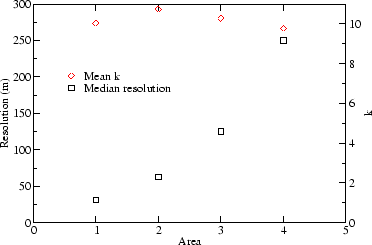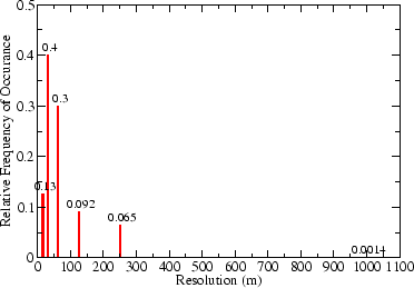
**Figure 3:** Dependency of spatial resolution and mean anonymity on area characteristics. For each evaluation area, the figure shows the median resolution from a large number of requests (left y-axis scale) and the mean *actual* anonymity--the number of subjects indistinguishable from the requestor (right y-axis scale).
$\begin{figure}\centerline{\psfig{figure=areasummary.eps,width=3.25in}}\end{figure}$

Figure 4 and Figure 5 provide more detail on the spatial resolution results by showing the relative distribution of resolutions in the form of histograms for a highway (1) and a collector area (4), respectively. While in the highway area less than 10% of requests reach a resolution lower than 125 meters, it is about 60% for the collector street area. Figure 5 also illustrates the relationship between anonymity and resolution in a single area. For lower resolutions (bigger areas) the mean anonymity does not stay near the minimum, but increases to more than triple the k_min constraint of five. When the algorithm is forced to choose a lower resolution, it has to quadruple the area and thereby includes more vehicles than necessary.

**Figure 4:** Relative frequency of spatial resolution for highway area (1). This figure illustrates the distribution of resolutions over a large number of simulated requests.
$\begin{figure}\centerline{\psfig{figure=I76k5adj.eps,width=3.25in}}\end{figure}$

**Figure 5:** Relative frequency of spatial resolution for collector road area (4). In addition to the distribution of resolutions (left y-axis scale), the figure shows the mean actual anonymity at each resolution (right y-axis scale).
$\begin{figure}\centerline{\psfig{figure=eofmarketk5adj.eps,width=3.25in}}\end{figure}$

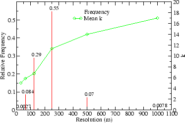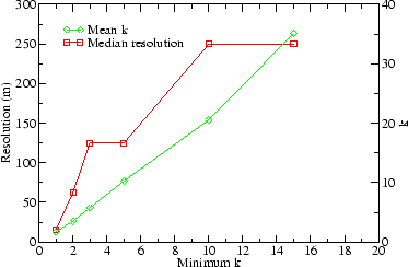
Figure 6 illustrates the tradeoff between the degree of anonymity and resolution, showing median resolution and mean anonymity k for different anonymity constraints k_min. The results stem from area number 3 with predominantly collector streets. Resolution is negatively correlated to the anonymity constraint. Also note that mean anonymity is approximately double the anonymity constraint. Again, this suggests that an improved discretization algorithm could yield better resolution with lower mean anonymity (i.e., closer to the minimum constraint).

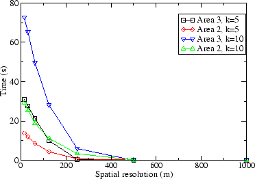
**Figure 6:** Dependency of spatial resolution and mean anonymity on anonymity constraint. This figure illustrates how spatial resolution (left scale) and mean actual anonymity (right scale) vary with different anonymity constraints (x-axis).
$\begin{figure}\centerline{\psfig{figure=kresults.eps,width=3.25in}}\end{figure}$

Spatial resolution can also be improved through reductions in temporal accuracy. Figure 7 shows the mean reduction in temporal resolution (and delay of messages) required to reach a specified spatial resolution. Results are reported for a highway area (2) and a collector street area (3). The anonymity constraint is also varied between five and ten. As expected, the temporal accuracy decreases for higher anonymity constraints, more collector streets, and higher spatial resolution. For highways the temporal resolution stays below 30s for resolutions up to 15m. On collector streets the resolution decreases to about 70s at this level of spatial accuracy.

**Figure 7:** Tradeoff between temporal and spatial resolution. The figure shows the mean reduction in temporal resolution necessary to reach a specified spatial resolution. The tradeoff is shown for a highway (2) and a collector (3) area at different anonymity constraints.
$\begin{figure}\centerline{\psfig{figure=temporal.eps,width=3.25in}}\end{figure}$