| ||||||||||||||||||||||||||||||||||||||||||||||||||||
|
JVM '02 Paper
[JVM '02 Tech Program Index]
To Collect or Not To Collect?Machine Learning for Memory Management
ABSTRACT
In this project we have researched an adaptive decision process that makes decisions regarding which garbage collector technique should be invoked and how it should be applied. The decision is based on information about the memory allocation behavior of currently running applications. The system learns through trial and error to take the optimal actions in an initially unknown environment. 1 IntroductionJRockit™, the Java™ Virtual Machine (JVM) constructed by Appeal Virtual Machines and now owned by BEA and named Weblogic JRockit, was designed recognizing that all applications are different and have different needs. Thus, a garbage collection technique and a garbage collection strategy that works well for one particular application may perform poorly for another. To achieve good performance over a broad spectrum of different applications, various garbage collection techniques with different characteristics have been implemented. However, any garbage collection technique requires a strategy that allows it to adapt its behavior to the current context of operation. Over the past few years, the need for better and more adaptive strategies has become apparent.Imagine that a JVM is running a program X. For this program, it might be best to garbage collect according to a rule Y. Whenever Y becomes true, the JVM garbage collects. However, this might not be the optimal strategy for another program X'. For X', rule Y' might be the best choice. Combining rule Y and Y' does not have to be complicated, but consider writing a combined rule that works really well for hundreds of programs? How does the JVM implementer know that a rule that works really well for many programs doesn't perform badly on others? Providing startup parameters for controlling the rule heuristics is a good start but it cannot adapt over time to a dynamic environment that has different needs at different points of time. The idea is to let a learning decision process decide which garbage collector technique to use and how to use it, instead of static rules making these decisions during run time. The learning decision process selects among different kinds of state of the art garbage collection techniques in JRockit™, the one that is best suitable for the current application and platform. The objective for this investigation is to find out if machine learning is able to contribute to improved performance of a commercial product. Theoretically machine learning could contribute to more adaptive solutions, but is such an approach feasible in practice? This paper is concerned with the question whether and, if so, how a learning decision process can be used for a more dynamic garbage collection in a modern JVM, such as JRockit. 1.1 Paper OverviewSection 2 relates the paper to previous work and in Section 3 we present the problem specification. Section 4 provides a survey of the reinforcement learning method that has been used. Section 5 presents possible situations of a system that uses a garbage collector in which a learning decision process might perform better than a regular garbage collector. Section 6 handles the design of the prototype and is followed by a presentation of experimental results, discussion of future developments and conclusions in Section 7, 8 and 9.2 Related workTo our current best knowledge we are not aware of any other attempt to utilize reinforcement learning in a JVM. Therefore, we are not able to provide references to similar approaches for that particular problem. Many papers on garbage collection techniques include some sort of heuristics on when the technique should be applied, but they are usually quite simple. These methods are usually straightforward and based on general rules that do not take the specific characteristics of the application into account.Brecht et al. [7] provide an analysis on when garbage collection should be invoked and when the heap should be expanded in the context of a Boehm-Demers-Weiser (BDW) collector. However, they do not introduce any adaptive learning but instead investigate the characteristic properties of different heuristics. 3 Problem SpecificationThe problem to solve is: how to design an automatic and learning decision process for more dynamic garbage collection in a modern JVM.Unlike some other garbage collection techniques, such as parallel garbage collection and stop-and-copy, concurrent garbage collection starts to garbage collect before the memory heap is full. A full heap would cause all application threads to stop, which would not be necessary if the concurrent garbage collector had started in time, since a concurrent garbage collector allows running applications to run concurrently with some phases of the garbage collection. For further reading about garbage collection, see references [2, 6, 8, 9, 13, 14]. An important issue, when it comes to concurrent garbage collection in a JVM, is to decide when to garbage collect. Concurrent garbage collection must not start too late, or else the running program may run out of memory. Neither must it be invoked too frequently, since this causes more garbage collections than necessary and thereby disturbs the execution of the running program. The key idea in our approach is to find the optimal trade-off between time and memory resources by letting a learning decision process decide when to garbage collect [2, 6, 8, 9, 13, 14]. 4 Reinforcement LearningReinforcement learning methods solve a class of problems known as Markov Decision Processes (MDP). If it is possible to formulate the problem at hand as an MDP, reinforcement learning provides a suitable approach to its solution [3, 4, 5].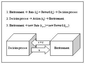
Figure 1 The figure shows model of a reinforcement learning system. First the decision process observes the current state and reward then the decision process performs an action that effects the environment. Finally the environment returns the new state and the obtained reward. Figure 1 depicts the interaction between an agent and its environment in a typical reinforcement learning setting. The agent perceives the current state of the environment by means of the state signal st upon which it responds with a control action at. More formally, a policy is a mapping from states to actions p: SxA --> [0, 1], in which p(s, a) denotes the probability with which the agent chooses action a in state s. As a result of the action taken by the agent in the previous state, the environment transitions to a new state st+1. Depending on the new state and the previous action the environment might pay a reward to the agent. The scalar reward signal indicates how well the agent is doing with respect to the task at hand. However, reward for desirable actions might be delayed, leaving the agent with the temporal credit assignment problem of figuring out which actions lead to desirable states of high rewards. The objective for the agent is to choose those actions that maximize the sum of future discounted rewards: R = rt + g rt+1 + g2 rt+2 …. The discount factor g[0,1] favors immediate rewards over equally large payoffs to be obtained in the future, similar to the notion of an interest rate in economics [1, 3, 5]. Notice, that usually the agent knows neither the state transition nor the reward function, neither do these functions need to be deterministic. In the general case the system behavior is determined by the transition probabilities P(st+1 | st, at) for ending up in state st+1 if the agent takes action at in state st and the reward probabilities P(r | st, at) for obtaining reward r for the state action pair st, at. A state signal that succeeds in retaining all relevant information about the environment is said to have the Markov property. In other words, in an MDP the probability of the next state of the environment only depends on the current state and the action chosen by the agent, and does not depend on the previous history of the system [1, 3, 5]. A reinforcement learning task that satisfies the Markov property is an MDP. More formally: if t indicates the time step, s is the state of the environment, a is an action taken by the agent and r is a reward, then the environment and the task have the Markov property if and only if [5]: Pr{st+1 = s’, rt+1 = r | st, at} is equal to: Pr{st+1 = s’, rt+1 = r | st, at, rt, st-1, at-1,…, r1, s0, a0} If it is possible to define a way of representing states such that all relevant information for making a decision is retained in the current state, the garbage collection problem becomes an MDP. Therefore, a prerequisite for being able to use reinforcement learning methods successfully is to find a way to represent states in a correct manner [1, 3, 5]. In theory it is required that the agent has complete information about the state of the environment in order to be able to guarantee asymptotic convergence to the optimal solution. However, often fast learning is much more important than a guarantee of eventually optimal performance. In practice, many reinforcement learning schemes are still able to achieve a good behavior in a reasonable amount of time even if the Markov property is violated [10]. Whereas dynamic programming requires a model of the environment for
computing the optimal actions, reinforcement learning methods are model
free and the agent obtains knowledge about its environment through interaction.
The agent explores the environment in a trial and error fashion, observing
the rewards obtained of taking various actions in different states. Based
on this information the agent updates its beliefs about the environment
and refines its policy that decides what action to take next [4, 5].
4.1 Temporal-Difference LearningThere are mainly four different approaches to solve Markov decision processes: Monte Carlo, temporal-difference, actor-critic and R-learning. For further discussion about these methods, see references [5, 6, 12, 15].What distinguishes temporal-difference learning methods from the other methods is that they update their beliefs at each time step. In application environments where the memory allocation rate varies a lot over time, it is important to observe the amount of available memory at each time step. Hence temporal-difference learning seems to be well suited for solving the garbage collecting problem [3, 5, 11, 15]. Temporal-difference learning is based on a value function, referred to as the Q-value function, which calculates the value of taking a certain action in a certain state. The algorithm performs an action, observes the new state and the achieved reward at each time step. Based on the observations, the algorithm updates its beliefs – the policy – and thereby theoretically improves its behavior at each time step [3, 5, 11, 15]. There are mainly two different approaches when it comes to temporal-difference methods: Q-learning and SARSA (State, Action, Reward, new State, new Action). This project has investigated the SARSA approach, since it is an on-policy method. On-policy means updating the policy that is being followed, i.e. the policy improves while being used. Further issues regarding how to use this method are discussed below. 4.2 Exploring vs. ExploitingIn reinforcement learning problems the agent is confronted with a trade-off between exploration and exploitation. On the one hand it should maximize its reward by always choosing the action a = maxa Q(s, a’) that has the highest Q-value in the current state s. However, it is also important to explore other actions in order to learn more about the environment. Each time the agent takes an action it faces two possible alternatives. One is to execute the action that according to the current beliefs has the highest Q-value. The other possibility is to explore a non-optimal action with a lower expected Q-value of higher uncertainty. Due to the probabilistic nature of the environment, an uncertain action of lower expected Q-value might ultimately turn out to be superior to the current best-known action. Obviously there is a risk, that the taking of the sub-optimal action diminishes the overall reward. However, it still contributes to the knowledge about the environment, and therefore allows the learning program to take better actions with more certainty in the future [4, 5, 11, 12].There are three different types of exploration strategies for choosing actions, the greedy algorithm, the e-greedy algorithm and the soft-max algorithm. The greedy algorithm is not of interest to use, since the garbage collection problem requires exploration. Both the other two algorithms are well suited for the garbage collection problem. However, the e-greedy algorithm was the choice we made. The e-greedy algorithm chooses the calculated, best action most of the times, but with a small probability e a random action is selected instead. The probability of choosing a random action is decreased over time and hence satisfies both needs for exploration and exploitation [1, 5]. 4.3 GeneralizationAnother common problem is environments that have continuous, and consequently infinitely many states. In this case it is not possible to store state-action values (Q-values) in a simple look-up table. A look-up table representation is only feasible when states and actions are discrete and few. Function approximation and generalization are solutions to this problem [3, 12].Generalization is a way of handling continuous values of state features. As it is the case of the garbage collection problem, generalization of the state is needed. Alternative approaches, other than generalization, to approximate the Q-value function are regression methods and neural networks [4, 6]. However, the approach used during this project was generalization. There are mainly four approaches for generalizing states and actions: coarse coding, tile coding, radial basis functions and Kanerva coding. For further reading about these methods see references [3, 5, 6]. Coarse coding is a generalization method using a binary vector, where each index of the vector represents a feature of the state, either present (1) or absent (0). Tile coding is a form of coarse coding where the state features are grouped together in partitions of the state space. These partitions are called tilings, and each element of a partition is called a tile. The more tilings you have, the more states will be affected of the reward achieved and share the knowledge obtained from an action performed. On the other hand, the system will get exponentially more complex depending on how many tilings are used [3, 5]. Tile coding is particularly well suited for use on sequential digital computers and for efficient online learning and is therefore used in this project [5]. 5 State Features and Actions of the General Garbage Collection ProblemIn the sections below some state features, actions and underlying reward features, possible to apply in a memory management system, are presented. Discussions of how they may be represented are also provided.5.1 Possible State FeaturesA problem in defining state features and rewards for a Markov decision process, is the fact that the evolution of the state to a large extent is governed by the running application as it determines which objects on the heap are no longer referenced and how much new memory is allocated. The garbage collector can only partially influence the amount of available memory in that it reduces fragmentation of the heap and frees the memory occupied by dead objects. Therefore, it is often difficult to decide whether to blame the garbage collecting strategy or the application itself for exceeding the available memory resources.In the following sections we present some suggestions of possible state features. Some state features might be difficult to calculate accurately at run time. For example, if the free memory were distributed across several lock-free caches, the number of free bytes would be hard to measure, or would at least take prohibitively long time to measure correctly. We therefore have to assume that approximations of these parameters are still accurate enough to achieve a reasonably good behavior. A fragmentation factor that indicates what fraction of the heap is fragmented is of interest. Fragments are chunks of free memory that are too small (<2kB) to belong to the free-list, from which new memory is allocated. As the heap becomes highly fragmented, garbage collection should be performed more frequently. This is desirable as it might reduce fragmentation by collecting dead objects adjacent to fragments. As a result, larger blocks of free memory may appear that can be reused for future memory allocation. In other words garbage collection should be performed when the heap contains a large number of non-referenced, small blocks of free memory. It is important to keep track of how much memory is available in the heap. Based on this information the reinforcement learning system is able to decide at which percentage of allocated memory it is most rewarding to perform a certain action, for instance to garbage collect. If the rate at which the running program allocates memory can be determined,
it would be possible to estimate at what point in time the application
will run out of memory, and hence when to start garbage collection at the
latest.
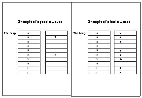
The average size of newly allocated objects might provide valuable information about the application running that can be utilized by the garbage collector. Another feature of the same category is the average age of newly allocated objects, if measurable. The amount of newly allocated objects is another possible feature. 5.2 State RepresentationEach observable system parameter, described in the previous section, constitutes a feature of the current state. Tile coding, see Section 4.3, is used to map the continuous feature values to discrete states. Each tiling partitions the domain of a continuous feature into tiles, where each tile corresponds to an interval of the continuous feature.The entire state is represented by a string of bits, with one bit per tile. If the continuous state value falls within the interval that constitutes the tile, the corresponding bit is set to ‘one’, otherwise it is set to ‘zero’: · The tile contains the current state feature value --> 1 · The tile does not contain the current state feature value --> 0 For example, a particular state is represented by a vector s = [1, 1, 0, …, 1, 0, 1], where each bit denotes the absence or presence of the state feature value in the corresponding tile. 5.3 Possible RewardsTo evaluate the current performance of the system, quantifiable values of the goals of the garbage collector are desired. The objectives of a garbage collector (see references [6, 9, 13 14]) concern maximization of the end-to-end performance and minimization of long interruptions of the running application, caused by garbage collection. These goals provide the basis for defining the appropriate scalar rewards and penalties.A necessity when deciding the reward function is to decide what are good and bad states or events. In a garbage-collecting environment there are a lot of situations that are neither bad nor good per se but might ultimately lead to a bad (or good) situation. This dynamic aspect adds another level of complexity to the environment. It is in the nature of the problem that garbage collection always intrudes on the process time of the running program and always constitutes extra costs. Therefore, no positive rewards are given but all reinforcement signals are penalties for consuming computational resources for garbage collection or even worse: running of out of memory. The objective of the learning process is to minimize the discounted accumulated penalties incurred over time. A fundamental rule for imposing penalty is to punish all activities that consume processing time from the running program. For instance a punishment is imposed every time the system performs a garbage collection. An alternative is to impose a penalty proportional to the fraction of time spent on garbage collection compared to the total run time of the program. Another penalty criterion is to punish the system when the average pause time exceeds an upper limit that is considered still tolerable by the user. It is also important to assure that the number of pauses does not exceed the maximum allowed number of pauses. If the average pause time is high and the number of pauses is low, the situation may be balanced by taking less time-consuming actions more frequently. If they are both high, a penalty might be in order. When using a concurrent collector, a severe penalty must be imposed if the running program runs out of memory and as a result has to wait until a garbage collection is completed, since this is the worst possible situation to arise. At first, it seems like a good idea to impose a penalty proportional to the amount of occupied memory. However, even if the memory is occupied up to 99 % this does not cause a problem, as long as the running application terminates without exceeding the available memory resources. In fact, this is the most desirable case, namely that the program terminates requiring no garbage collection but still never runs out of memory. Therefore, directly imposing penalties for the occupation of memory is not a good idea. The ratio of freed memory after completed garbage collection compared
to the ratio allocated memory in the heap prior to garbage collection provides
another possible performance metric. This parameter gives an estimate of
how much memory has been freed. If the amount is large there is nothing
to worry about, as illustrated to the left in Figure 2. If the amount freed
memory is low and the size of the free-list is low as well, problems may
occur and hence the garbage collector should be penalized. The latter situation,
illustrated to the right in Figure 2, might occur if a running program
has a lot of long-living objects and runs for a long time, so that most
of the heap will be occupied.
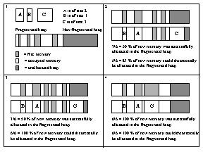
When using compacting garbage collectors, it is interesting to observe
the success rate of allocated memory in the most fragmented area of the
heap. The actual amount of new memory allocated in the fragmented area
of the heap is compared to the theoretical limit of available memory in
case of no fragmentation at all. An illustration of some possible situations
is shown in Figure 3. It is desirable that 100 % of the newly allocated
memory is allocated in the most fragmented area of the heap, in order to
reduce fragmentation. A penalty is imposed that is inversely proportional
to the ratio of actual allocated memory and its theoretical limit in the
best possible case.
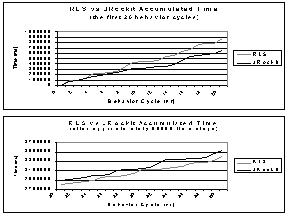
If the memory relies on global structures that need a lock to be accessed, taking the lock ought to be punished. This might be the case for memory free-lists, caches etc. The more time a compacting garbage collector spends on iterating over the free-list (for explanation see references [13, 14]) the more it should be penalized. A long garbage collection cycle is an indicator for a fragmented heap. High fragmentation in itself is not necessarily bad, but the iteration consumes time otherwise available to the running application, which is why such a situation should be punished. When it comes to compacting garbage collectors a measurement of the effectiveness of a compaction provides a possible basis for assigning a reward or a penalty. If there was no need for compacting, the section in question must have been non-fragmented. Accordingly a situation like this should be assigned a reward. There is one possible desirable configuration to which a reward, rather than a penalty, should be assigned, namely if a compacting collector frees large, connected chunks of memory. The opposite, if the garbage collector frees a small amount of memory and the running program is still allocating objects, could possibly be punished in a linear way, as some of the other reward situations described above. 5.4 Possible ActionsWhether to invoke garbage collection or not at a certain point of time is the most important decision for the garbage collecting strategy to take. Therefore, the set of possible actions taken by the prototype discussed in the later section is reduced to this binary decision.When the free memory is not large enough and the garbage collection fails to free a sufficiently large amount of memory, a possible remedy is to increase the size of the heap. It is also of interest to be able to decrease the heap size, if a large area of the heap never becomes allocated. To decide whether to increase or decrease the heap size can constitute an action. If a change is needed a complementary decision is to decide the new size of the heap. To save heap space or rather to use the available heap more effectively, a decision to compact the heap or not, could also be of interest. In addition the action could specify how much and which section of the heap to compact. To handle synchronization between allocating threads of the running program, a technique of using lock-free Thread Local Areas (TLAs) is usually used. Each allocating thread is allowed to allocate memory within only one TLA at a time and vice versa there is only one thread permitted to allocate memory in a particular TLA. The garbage collection strategy could determine the size of each TLA and how to distribute the TLAs between the threads. When allocating large objects often a Large Object Space (LOS) is used, especially in cases where generational garbage collectors are considered, in order to avoid moving large objects. Deciding the size of the LOS and how large an object has to be, to be considered a large object, are additional issues for the reinforcement learning decision process to consider. To reduce garbage collection time, smaller free blocks might not be added to a free list during a sweep-phase. The memory block size is the minimum size of a free memory block for being added to the free list. Different applications may have different needs with respect to this parameter. How many generations are optimal for a generational garbage collector? With the current implementation it is only possible to decide prior to starting the garbage collector if it operates with either one or two generations. It might be possible, even today, to reduce the number of generations from two to one, but not to increase them during run-time. When it comes to future generational garbage collectors it would be of interest to let the system vary the size of the different generations. If there is a promotion rate available, this is a factor that might be interesting for the system to vary as well. If the garbage collector uses an incremental approach, deciding the size of the heap area that is collected at a time might be an interesting aspect to consider. The same applies to deciding whether to use the concurrent approach, in conjunction with the factors of how many garbage collection steps to perform at a time and how long a time the system should pre-clean (for explanation see references [14]). 6 The PrototypeThe state features used in the prototype are the current amount of available memory, s1, and the change in available memory, s2, calculated as the difference between s1 at the previous time step - s1 at the current time step.There is only one binary decision to make, namely whether to garbage collect or not. Hence, the action set contains only two actions {0, 1}, where 1 represents performing a garbage collection and 0 represents not performing a garbage collection. The tile coding representation of the state in the prototype was chosen to be one 10x2-tiling in the case where only s1 was used. In the case where both state features were used the tile coding representation was chosen to be one 10x7x2-tiling, one 10-tiling, one 7-tiling and one 10x7-tiling. A non-uniform tiling was chosen, in which the tile resolution is increased for states of low available memory, and a coarser resolution for states in which memory occupancy is still low. The tiles for feature s1 correspond to the intervals [0, 4], [4, 8], [8, 10], [10, 12], [12, 14], [14, 16], [16, 18], [18, 20], [22, 26] and [30, 100]. The tiles for feature s2 are at a resolution: [<0], [0-2], [3-4], [5-6], [7-8], [9-10] and [>10]. The reward function of the prototype imposes a penalty (-10) for performing a garbage collection. The penalty for running out of memory is set to -500. It is difficult to specify the quantitative trade-off between using time for garbage collection and running out of memory. In principle the later situation should be avoided at all costs, but a too large penalty in that case might bias the decision process towards too frequent garbage collection. Running out of memory is not desirable since a concurrent garbage collector is used. A concurrent garbage collector must stop all threads if the system runs out of memory, which is the major purpose of using a concurrent garbage collector in the first place. The probability p that determines whether to pick the action with the highest Q-value or a random action for exploration evolves over time according to the formula: p = p0 * e -(t / C) where p0 = 0.5 and C = 5000 in the prototype, which means that random actions are chosen with decreasing probability until approximately 25000 time steps elapsed. A time step t corresponds to about 50ms of real time between two decisions of the reinforcement learning system. The learning rate a decreases over time according to the formula stated below: a = a0 * e -(t / D) where a0 = 0.1 and D = 30000 in the prototype. The discount factor g is set to 0.9. The test application used for evaluation is designed to demonstrate a very dynamic memory allocation behavior. The memory allocation rate of the test application alternates randomly between different behavior cycles. A behavior cycle consists of either 10000 iterations or 20000 iterations of either low or high memory allocation rate. The time performance of the RLS is measured during a behavior cycle as the number of milliseconds required to complete the cycle. 6.1 Interesting Comparative MeasurementsThe performance of the garbage collector in JRockit ought to be compared to the performance when using the reinforcement system for deciding when to garbage collect not only in terms of time performance but also in terms of the reward function. The reward function is based on the throughput and the latency of a garbage collector and the underlying features of the reward function are hence suitable for extracting comparable results of the two systems.However, learning a proper garbage collection policy should take a reasonable amount of time, as otherwise the reinforcement learning system would be of little practical value. The first step of an evaluation of RLS is to verify that learning and adaptation actually occur at all, namely that the system improves its performance over time. The learning success is measured by the average reward per time step. Analyzing the time evolution of the Q-function provides additional insight into the learning progress. 7 ResultsOne of the main objectives of this project is the identification of suitable state features, underlying reward features and action features for the dynamic garbage-collection learning problem. An additional objective is the implementation of a simple prototype and the evaluation of its performance on a restricted set of benchmarks in order to investigate whether the proposed machine learning approach is feasible in practice.This section compares the performance of a conventional JVM with a JVM using reinforcement learning for making the decision: when to garbage collect. The JVM using reinforcement learning is referred to as the RLS (Reinforcement Learning System) and the conventional JVM is JRockit. Since JRockit is optimized for environments in which the allocation behavior changes slowly, environments where the allocation behavior changes more rapidly might cause a degraded performance of JRockit. In these environments it is of special interest to investigate if an adaptive system, such as an RLS, is able to perform equally well or even better than JRockit. Figure 4 shows the results of using the RLS and JRockit for the test
application described in Section 6. Due to the random distribution of behavior
cycles a direct cycle-to-cycle comparison of these two different runs is
not meaningful. Instead, the accumulated time performances, illustrated
in Figure 4, are used for comparison. As may be seen in the lower chart,
the RLS performs better than JRockit in this dynamic environment. This
confirms the hypothesis of an RLS being able to outperform an ordinary
JVM in a dynamic environment.
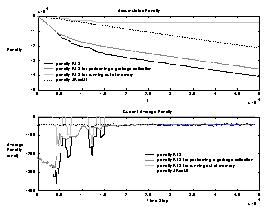
Figure 5 illustrates the accumulated penalty for the RLS compared to
JRockit. In the beginning the RLS runs out of memory a few times, as shown
in the graph labeled penalty RLS for running out of memory, but after about
15000 time steps it learns to avoid running out of memory. The lower chart
shows the current average penalty of the RLS and JRockit. After about 20000
time steps the RLS has adapted its policy and achieves the same performance
as JRockit. The results show that the RLS in principle is able to learn
a policy that can compete with the performance of JRockit. The test session
only takes about an hour, which is a reasonable learning time for offline
learning (i.e. following one policy while updating another) of long running
applications. Also, no attempt has been made to optimize the parameters
of the RLS, such as exploration and learning rate, in order to minimize
learning time within this project.
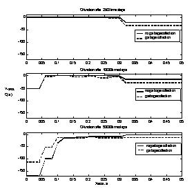
The accumulated penalty over a time period between time step 30000 and 50000 after RLS completed learning, has been calculated to -8400. The corresponding accumulated penalty for JRockit for the same period of time was calculated to -8550. This shows that the results of the RLS are comparable to the results of JRockit. The values verify the results presented above: that the RLS performs equally well or even slightly better than JRockit in an intentionally dynamic environment. In the following we analyze the learning process in more detail by looking at the time evolution of the Q-function for the single feature case that only considers the amount of free memory. The upper chart in Figure 6 compares the Q-function for both actions, namely to garbage collect or not to garbage collect, after approximately 2500 time steps. Notice, that the RLS always prefers the action of higher Q-value. The probability p of choosing a random action is still very high and garbage collection is randomly invoked frequently enough to prevent the system from running out of memory. On the other hand the high frequency of random actions during the first 5000 time steps leads the system to avoid deliberate garbage collection action at all. In other words it always favors not to garbage collect in order to avoid the penalty of -10 units for the alternative action. Initially, the system does not run out of memory due to the high frequency of randomly performed garbage collections. The only thing the system has learned so far is that it is better not to garbage collect than to garbage collect. Notice, that the system did not learn for states of low free memory, as those did not occur yet. The difference of the Q-value between the two actions is -10, which corresponds exactly to the penalty for performing a garbage collection. This makes sense insofar as the successor state after performing a garbage collection is similar to the state prior to garbage collection, namely a state for which the amount of memory available is still high. The middle chart in Figure 6 shows the Q-function after approximately 10000 time steps. The probability of choosing a random action has now decreased to the extent, that the system actually runs out of memory. Once that happens the RLS incurs a large penalty, and thereby learns to deliberately take the alternative action, namely to garbage collect at states of low available memory. The lower chart in Figure 6 illustrates the Q-function after approximately
50000 time steps. At this point the Q-values for the different states has
already converged. Garbage collection is invoked once the amount of available
memory becomes lower than approximately 12%. This policy is optimal considering
the limited state information available to RLS, the particular test application
and the specific reward function.
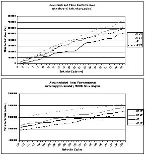
The performance comparison between the RLS and JRockit suggests further investigation of reinforcement learning for dynamic memory management. Regarding the fact that this first version of the prototype only considers a single state feature, it would be interesting to investigate the performance of an RLS that takes additional and possibly more complex state features into consideration. Additional state features might enable the RLS to take more informed decisions and thereby achieve even better performance. In Figure 7 the accumulated time performance of the RLS using one (1F2T) and two state features (2F5T), and JRockit (JR) is compared. In the case of two state features, five (instead of only two) tilings were used in order to achieve better generalization across the higher dimensional state space. In order to illustrate the effect of five tilings, the time performance of an RLS using two state features but only two tilings (2F2T) is also shown in the charts of Figure 7. The upper chart illustrates the performance of the four systems in the initial stage at which the RLS is adapting its policy. The lower chart shows the performance after approximately 50000 decisions (time steps). The graphs show that the RLS using two state features and five tilings does not perform better than the RLS using only one state feature or JRockit. However, the system using five tilings is significantly better than the RLS using two state features and two tilings. The main reason for the inferior behavior is probably that the new feature
increases the number of states and that therefore converging to the correct
Q-values and optimal policy requires more time. The decision boundary is
more complex than in the case of only a single state feature. The number
of states for which the RLS has to learn that it runs out of memory, if
it does not perform a garbage collection, has increased and thereby also
the complexity of the learning task.
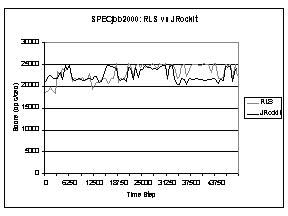
Another consequence of the increased number of states is that the system runs out of memory more often. To some extent Q-function approximation (i.e. tile coding, function approximation) provides a remedy to this problem. Further investigation regarding this aspect is needed, see the discussion in Section 8. To provide some standard measurement results the best RLS, i.e. the
RLS using only one state feature, is compared to the JRockit version used
in previous test sessions due to SPECjbb2000 scores. In Figure 8 the results
of a test session with full occupancy from the beginning are presented.
As mentioned before, the RLS is learning until the 30000th time step (decision).
The average performance scores of both systems are presented in Table 1. As may be observed, the use of the RLS for the decision of when to garbage collect improves the average performance by 2%. That number already includes the learning period. If the learning period of the RLS is excluded (i.e. measured after approximately 30000 decisions), the average improvement when using the RLS is 6%. Table 1 The table illustrates the average performance results of the RLS using one state feature and JRockit, when running SPECjbb2000 with full occupancy.
8 Discussion and Future DevelopmentsThe preliminary results of our study indicate that reinforcement learning might improve existing garbage collection techniques. However, a more thorough analysis and extended benchmark tests are required for an objective evaluation of the potential of reinforcement learning techniques for dynamic memory management.The most important task of future investigation is to systematically investigate the effect of using additional state features for the decision process and to investigate their usefulness for making better decisions. The second important aspect is to investigate more complex scenarios of memory allocation, in which the memory allocation behavior switches more rapidly and less regularly. It is also of interest to investigate other dimensions of the garbage-collection problem such as object size and levels of references between objects, among others. It is important to emphasize that the results above are derived from a limited set of test applications that cannot adequately represent the range of all possible applications. The issue of selecting proper test application environ-ments also relates to the problem of generalization. The question is: how much does training on one particular application or a set of multiple applications help to perform well on unseen applications? It would be interesting to investigate how long it takes to learn from scratch or how fast an RLS can adapt when the application changes dynamically. Another suggestion for improving the system is to decrease the learning rate more slowly. The same suggestion applies to the probability of choosing a random action in order to achieve a better balance between exploitation and exploration. The optimal parameters are best determined by cross-validation. An approach for achieving better results when more state features are taken into account might be to represent the state features in a different way. For instance, radial basis functions, mentioned earlier in this report, might be of interest for generalization of continuous state features. An even better approach would be to represent the state features with continuous values and to use a gradient-descent method for approximating the Q-function. It seems that that the total number of state features is a crucial factor. JRockit considers only one parameter for the decision of when to garbage collect. The performance of the RLS was not improved using two state features, likely due to the enlarged state space. The question remains, whether the performance of the RLS improves if additional state information is available and the time for exploration is increased. The potential strength of the RLS might reveal itself better if the decision is based on more state features than JRockit uses currently. Another important aspect is online vs. offline performance. How much learning can be afforded, or shall only online-performance be considered? That of course is also a design issue for JRockit, which relies on a more precise definition of the concrete objectives and requirements of a dynamic Java Virtual Machine. Once a real system has been developed from the prototype, it can be used to handle some of the other decisions related to garbage collection proposed in this report. It is recommended to investigate this research area further, since it is far from exhausted. Considering that the results were achieved using a prototype that is poorly adjusted in several aspects, further development might lead to interesting and even better results than obtained within the restricted scope of this project. 9 ConclusionsThe trade-off that every garbage collecting system faces is that garbage collection in itself is undesirable, as it consumes time from the running program. However, if garbage collection is not performed the system runs the risk of running out of memory, which is far worse than slowing down the application. The motivation for using a reinforcement learning system is to optimize this trade-off between saving CPU time and avoiding exhaustion of the memory.This report has investigated how to design and implement a learning decision process for a more dynamic garbage collection in a modern JVM. The results of this thesis show that it is in principle possible for a reinforcement learning system to learn when to garbage collect. It has also been demonstrated that on simple test cases the performance of the RLS after training in terms of the reward function is comparable with the heuristics of a modern JVM, such as JRockit. The time it takes for the RLS to learn also seems reasonable since the system only runs out of memory 5-10 times during the learning period. Whether this cost of learning a garbage collecting policy is acceptable in real applications depends on the environment and the requirements on the JVM. From the results in the case of two state features, it becomes clear that using multiple state features potentially results in more complex decision surfaces than simple standard heuristics. Observations have also been made that there exists an evident trade-off between using more state features, in order to make more optimal decisions, and the increased time required for learning due to an enlarged state space. From the above results one can learn that the use of a reinforcement learning system is particularly useful if an application has a complex dynamic memory allocation behavior, which is why a dynamic garbage collector was proposed in the first place. It is noteworthy to observe that machine learning through an adaptive and optimizing decision process can replace a human designed heuristic such as JRockit that operates with a dynamic threshold. This article is an excerpt of the project report Reinforcement Learning for a Dynamic JVM [6], which may be obtained by contacting the author at: eva.andreasson@appeal.se. 10 ReferencesLiterature1. Bertsekas, D. P. and Tsitsiklis, J. N. (1996). Neuro-dynamic programming. Athena Scientific, Belmont, Massachusetts, USA. 2. Jones, R. and Lins, R. (1996). Garbage collection – algorithms for automatic dynamic memory management. John Wiley & Sons Ltd., Chichester, England, UK. 3. Mitchell, T. M. (1997). Machine learning. McGraw Hill, USA. 4. Russell, S. J. and Norvig, P. (1995). Artificial intelligence – a modern approach. Prentice-Hall, Inc., Englewood Cliffs, New Jersey, USA. 5. Sutton, R. S. and Barto, A. G. (1998). Reinforcement learning – an introduction. MIT Press, Cambridge, Massachusetts, USA. Papers
|
|
This paper was originally published in the
Proceedings of the 2nd JavaTM Virtual Machine
Research and Technology Symposium, San Francisco, California, USA
August 1-2, 2002
Last changed: 22 July 2002 ml |
|