IMC '05 Paper
[IMC '05 Technical Program]
Poisson versus periodic path probing (or, does PASTA
matter?)
Muhammad Mukarram Bin Tariq, Amogh Dhamdhere,
Constantinos Dovrolis, Mostafa Ammar
Georgia Institute of Technology
{mtariq,amogh,dovrolis,ammar}@cc.gatech.edu
Abstract--
The well-known PASTA (``Poisson Arrivals See Time Averages'') property
states
that, under very general conditions, the fraction of Poisson arrivals
that observe an underlying process in a particular state is equal,
asymptotically, to the fraction of time the process spends in that
state. When applied to network inference, PASTA implies that a Poisson
probing stream provides an unbiased estimate of the desired time
average. Our objective is to examine the practical significance of the
PASTA property in the context of realistic RTT, loss rate and packet
pair dispersion measurements with a finite (but not small) number of
samples. In particular, we first evaluate the differences between the
point estimates (median RTT, loss rate, and median dispersion) that
result from Poisson and Periodic probing. Our evaluation is based on a
rich set of measurements between 23 PlanetLab hosts. The experimental
results show that in almost all measurement sessions the differences
between the Poisson and Periodic point estimates are insignificant. In
the case of RTT and dispersion measurements, we also used a
non-parametric goodness-of-fit test, based on the Kullback-Leibler
distance, to evaluate the similarity of the distributions that result
from Poisson and Periodic probing. The results show that in more than
90% of the measurements there is no statistically significant
difference between the two distributions.
1 Introduction
In the context of active measurements, a sequence of probing
packets is injected in a network path with the objective to measure
end-to-end properties such as Round-Trip Time (RTT), loss rate, or
available bandwidth (related to the time-spacing, or dispersion,
between successive packets).
A central issue in active measurements
is the characteristics of the probing process [1]. From a mathematical
perspective, it is often claimed that ``the right way'' to do probing
(or sampling) is to use a Poisson process (meaning that the
interarrivals between probing packets should be independent
and exponentially distributed with the same mean)
[2,3,4,5,6].
Poisson probing derives its strength from the well-cited PASTA
property, which stands for ``Poisson Arrivals See Time Averages'' [7].
Consider a stochastic system and
suppose that we want to infer the fraction of time  the
system spends in a state the
system spends in a state  . Let us assume that this time
average exists. A stream of . Let us assume that this time
average exists. A stream of  ``probes'' arrives
in the system based on a Poisson process, recording the system's state
at the arrival time instant. PASTA states that the expected value ``probes'' arrives
in the system based on a Poisson process, recording the system's state
at the arrival time instant. PASTA states that the expected value ![$E[f_{X,N}]$](img8.png) of the fraction of Poisson probes that observe the system
at state is equal to the time average .
This powerful result does not make any assumptions about the stochastic
system,
except that the time average exists; stationarity
or ergodicity may be needed in order to prove that however. of the fraction of Poisson probes that observe the system
at state is equal to the time average .
This powerful result does not make any assumptions about the stochastic
system,
except that the time average exists; stationarity
or ergodicity may be needed in order to prove that however.
The underlying reason for the validity of PASTA is that the
monitored system cannot ``anticipate'' the next probing
event, due to the memoryless nature of the Poisson measurement process.
Notice that the the Poisson probes may be interacting with the
monitored
system. In the case of a queueing system, for example, probing
packets can be backlogged, serviced, or dropped, as any other packet,
and they may also affect the magnitude of the time average . It is also important to note that PASTA is an asymptotic
result:
 tends to as the number of
probes tends to infinity.
The sample average , even though an unbiased estimate,
can significantly deviate around depending on and on the variability
and correlation structure of the underlying system [8]. tends to as the number of
probes tends to infinity.
The sample average , even though an unbiased estimate,
can significantly deviate around depending on and on the variability
and correlation structure of the underlying system [8].
On the practical side,
the most common measurement approach is to use Periodic
probing, rather than Poisson probing. For instance, the popular ping
utility generates a periodic probing stream.
An important advantage of Periodic probing is that the
duration of a measurement session can be a priori known,
given the number of samples and the probing period. Furthermore,
scheduling periodic packet transmissions
at mainstream (not real-time) operating systems is easier
and more accurate than scheduling random, and potentially very short
or very long, packet interarrivals.
It should be noted that the use of Periodic probing does
not mean that the resulting estimate will be necessarily
biased, especially if the probing rate is sufficiently high.
It is true, however, that only Poisson probing can provably result in
an unbiased estimate
under general conditions.
An important question, which is still unresolved to the best of our
knowledge, is whether PASTA ``matters'' in the pragmatic context
of RTT, loss rate, and bandwidth (or dispersion) measurements in the
Internet. Given that Periodic probing has some important practical
benefits, we need to know whether Poisson and Periodic probing
sequences
lead to significantly different estimates.
In this paper, we focus on three significant path performance metrics:
RTT, loss rate and dispersion of back-to-back packet pairs.
Our objective is to evaluate the differences that result from
Poisson and Periodic probing, both in terms of point estimates
for the first moment of the underlying distributions,
as well as in terms of differences in the distributions themselves.
Note that, since this is a measurement study over wide-area Internet
paths, we do not know whether Poisson and/or Periodic probing measure
the actual
time average of the previous performance metrics. Instead, we can only
examine whether the two probing techniques
observe the same (but potentially wrong!) path performance.
In Section 2, we
describe our measurement collection process.
In Sections 3, 4, and 5
we analyze the RTT, loss rate, and dispersion measurements,
respectively. Our results show that in almost all measurement sessions
the differences between Poisson and Periodic
point estimates are insignificant.
In the case of RTT and dispersion measurements,
there is no statistically significant difference between the Poisson
and Periodic distributions in about 90% of the measurements.
We conclude with some additional remarks in Section 6.
2 Measurement methodology
We collected measurements of RTT, packet loss rate, and packet pair
dispersion
in network paths between 23 PlanetLab hosts. Specifically, we used
PlanetLab nodes at the following sites:
RNP (Brazil), UC San Diego,
UC Berkeley, U-Oregon, U-British Columbia,
U-Texas,
UIUC,
Georgia Tech,
CMU,
MIT,
U-Maryland, INRIA (France),
Intel Research Cambridge (UK),
UPC (Spain),
U-Reykjavik (Iceland),
EPFL (Switzerland),
Helsinki Inst. of Tech. (Finland),
U-Tsinghua (China),
Hong Kong Univ. of Science & Tech,
National Taiwan Univ,
Equinix (Singapore),
U-Tokyo (Japan), and U-Melbourne (Australia).
The measurements reported in this paper were collected from
53 source-destination pairs.
Each measurement session (or simply ``session'') consists of
600 Poisson probes and 600 Periodic probes transmitted
at the same average rate. The two probing streams of a session
start at the same time, and so they cover approximately the same time
window.
A session is characterized by a source-destination pair, the average
probing interarrival  , and the packet size , and the packet size  .
The probing interarrival was 10ms, 20ms, 50ms, 100ms, 500ms, or 1sec,
meaning that a session lasts from 6 seconds to 10 minutes, depending on
.
For the RTT and loss rate sessions was 32, 64, 480, or
1400 bytes, while
for the dispersion measurements was 480, 800, or
1400 bytes.
The number of successfully completed sessions was 1272 for each of the
RTT and loss rate
measurements and 954 for the dispersion measurements. .
The probing interarrival was 10ms, 20ms, 50ms, 100ms, 500ms, or 1sec,
meaning that a session lasts from 6 seconds to 10 minutes, depending on
.
For the RTT and loss rate sessions was 32, 64, 480, or
1400 bytes, while
for the dispersion measurements was 480, 800, or
1400 bytes.
The number of successfully completed sessions was 1272 for each of the
RTT and loss rate
measurements and 954 for the dispersion measurements.
It turned out that some paths were either too slow for our probing
streams (especially with =10ms or 20ms and
large packet sizes), or they were extremely congested.
In a pre-processing step, we filtered out all sessions in which
the loss rate was higher than 10% in the RTT and dispersion analysis;
those sessions were included, however, in certain parts of the loss
rate analysis (as noted in § 4).
The number of sessions we were left with was 892 for RTT and loss rate
and 749 for dispersion.
The RTT and dispersion time measurements were obtained with
kernel-level (libpcap) timestamps, reported in a resolution of
one microsecond.
3 RTT measurements
Comparison of median RTTs:
The sample median is a robust point estimate for the first
moment of a distribution.
Let  and and  be the median RTTs
estimated from the Poisson and Periodic probing streams, respectively,
in a particular session.
We define the relative difference between the two RTT medians
as be the median RTTs
estimated from the Poisson and Periodic probing streams, respectively,
in a particular session.
We define the relative difference between the two RTT medians
as
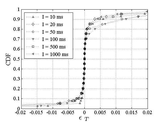
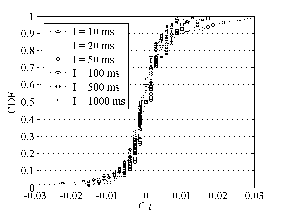
 . Figure 1 shows the empirical CDF of . Figure 1 shows the empirical CDF of  . About 60% of the sessions do not see any
difference
( . About 60% of the sessions do not see any
difference
(
 ), while about 85% of the sessions
have ), while about 85% of the sessions
have  1%.
The maximum relative difference is 4%. The results are actually quite
similar for the relative difference of RTT means.
Consequently, at least in relative error terms, Poisson and Periodic
probing result in practically the same RTT estimate.
The fact that the two probing processes measure almost equal median
RTTs, however, does not mean that they also observe the same RTT
distribution;
we examine this issue next. 1%.
The maximum relative difference is 4%. The results are actually quite
similar for the relative difference of RTT means.
Consequently, at least in relative error terms, Poisson and Periodic
probing result in practically the same RTT estimate.
The fact that the two probing processes measure almost equal median
RTTs, however, does not mean that they also observe the same RTT
distribution;
we examine this issue next.
Figure 1:
The relative difference between Poisson and
Periodic RTT medians.
|
|
Goodness-of-fit test: To further explore the differences between
Poisson and Periodic probing,
we also examine the RTT distributions measured by the two
probing processes.
Let  and and  be the Poisson and
Periodic RTT samples, respectively,
collected in a particular session.
We form the following null hypothesis: be the Poisson and
Periodic RTT samples, respectively,
collected in a particular session.
We form the following null hypothesis:
 |
(1) |
The alternate hypothesis is that there is a statistically significant
difference between the two distributions.
A non-parametric goodness-of-fit test can reject  with a low P-value when the two given samples
have
a statistically significant difference, even if the underlying
distributions
are strongly non-Gaussian. Recall that P-value is the lowest
significance level with a low P-value when the two given samples
have
a statistically significant difference, even if the underlying
distributions
are strongly non-Gaussian. Recall that P-value is the lowest
significance level  at which we can reject the null
hypothesis. The P-value is between 0 and 1. is often
rejected when the P-value is less than 0.05-0.10. at which we can reject the null
hypothesis. The P-value is between 0 and 1. is often
rejected when the P-value is less than 0.05-0.10.
Our initial approach was to use the well-known Kolmogorov-Smirnov
(KS) test. This test, however, assumes that the underlying
distributions
are continuous. Furthermore, it is quite sensitive to that
assumption
because it focuses on the maximum vertical distance between the two
empirical CDFs. It is important to note that the RTT distribution
at an Internet path can be almost discontinuous when several
probing
packets measure the same RTT value that is
determined by constant propagation and transmission delays.
This discontinuity is located at the minimum
(or close to the minimum) measurement, and it is more likely in lightly
loaded
paths with small queueing delays because the latter can only increase
the RTT measurements.
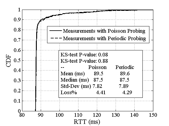
Figure 2:
A session in which the KS test performs poorly.
|
|
For example, Figure 2
shows the two RTT empirical CDFs measured in a session from MIT to
U-Oregon (=20ms, =480 bytes). Note
that for all practical purposes the two distributions are identical.
The KS test, however, rejects with a low P-value ( =0.08).
The reason the test fails is the discontinuity at about 87.5ms.
The maximum vertical distance between the two CDFs is 7.4%, it occurs
at the 25-th percentile of the Poisson distribution,
while the horizontal offset with the Periodic distribution
at that point is only 31 microseconds! It is noted that we observed
similar failures with other non-parametric statistical tests, such as
the Kruskal-Wallis analysis-of-variance test. =0.08).
The reason the test fails is the discontinuity at about 87.5ms.
The maximum vertical distance between the two CDFs is 7.4%, it occurs
at the 25-th percentile of the Poisson distribution,
while the horizontal offset with the Periodic distribution
at that point is only 31 microseconds! It is noted that we observed
similar failures with other non-parametric statistical tests, such as
the Kruskal-Wallis analysis-of-variance test.
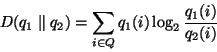
To deal with the previous discontinuity problems,
we constructed a more robust non-parametric goodness-of-fit test based
on the Kullback-Liebler (KL) distance, also known as relative
entropy [9].
For two discrete probability mass functions (pmf's)  and and  ,
defined over the same set of values ,
defined over the same set of values  ,
the KL distance of relative to is ,
the KL distance of relative to is
 |
(2) |
It can be shown that  and that and that
 if and only if the two distributions are identical.
Notice that if and only if the two distributions are identical.
Notice that  . .
The KL test proceeds in three steps:
- Estimate the pmf's
 and and  (defined on the same set of bins) from the samples and , respectively.
The details of the binning procedure are described in the Appendix. (defined on the same set of bins) from the samples and , respectively.
The details of the binning procedure are described in the Appendix.
- Calculate the KL distance
 of the Poisson relative to the Periodic
sample. of the Poisson relative to the Periodic
sample.
- Estimate the distribution of the KL distance
 between randomly
chosen partitions between randomly
chosen partitions  and and  of the Poisson sample
(``bootstrapping'').
Specifically, suppose that we randomly partition in two
samples and .
Let
of the Poisson sample
(``bootstrapping'').
Specifically, suppose that we randomly partition in two
samples and .
Let  and and  be the corresponding
pmf's, and so is the KL distance
of this partition. If we repeat this random partitioning process many
times, we can estimate the distribution of . be the corresponding
pmf's, and so is the KL distance
of this partition. If we repeat this random partitioning process many
times, we can estimate the distribution of .
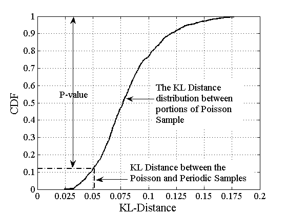
- Reject the null hypothesis if
is ``too large'' relative to the distribution
 . Specifically,
estimate the P-value as . Specifically,
estimate the P-value as
![\begin{displaymath}
P \approx \mbox{Prob}[D(s_e \parallel s_p) \leq D(s_{e,i} \parallel %
\bar{s}_{e,i})]
\end{displaymath}](img40.png) |
(3) |
and reject if  . .
Figure 3 shows an
example of the distribution
of together with the
KL distance for a particular session. The KL test is more
robust than the KS test
in the presence of CDF discontinuities. The reason is that
instead of relying on a single point of maximum vertical difference,
the KL test considers the difference between the two distributions
across all bins, weighted by the probability mass at each bin. For the
example of Figure 2,
the KL test
reports a P-value of 0.88, meaning that the null hypothesis
cannot be rejected.
Figure 3:
An example of the KL distance distribution for a particular session.
|
|
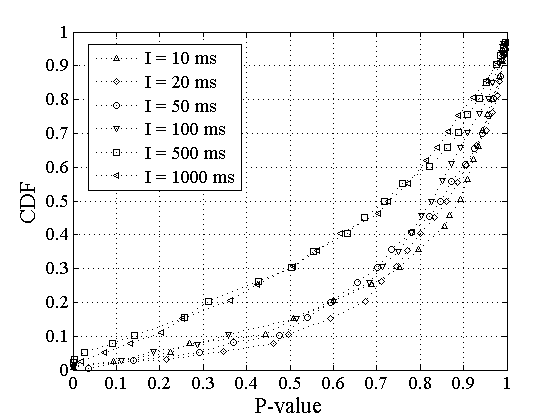
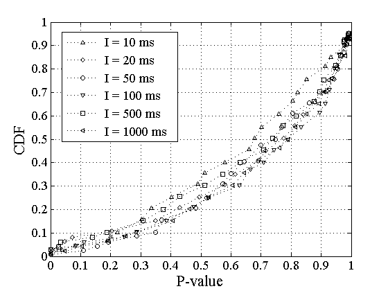
Figure 4:
Distribution of P-values for the null hypothesis ,
applied to RTT sessions.
|
|
Figure 4 shows the
distribution of P-values
reported by the KL test for various probing interarrivals .
We see that we can reject for only 5-10% of
the sessions
at a significance level of 10%.
The rest of the sessions have significantly higher P-values,
meaning that we cannot reject .
So, for more than 90% of the measurement sessions we can
assume that the RTT distributions observed by Poisson and Periodic
probing are identical.
Note that the two larger average probing periods, 500ms and 1000ms,
result in lower P-values, implying wider (but still not statistically
significant) differences between the two RTT distributions.
When is 500ms and 1000ms the measurement process
lasts for
300sec and 600sec, respectively, and the underlying process shows
significant variability during that time window. Consequently, the two
probing processes are more likely to observe
different values of the underlying process.
4 Loss rate measurements
For the loss rate estimates, we used the same set of sessions
as in the case of RTTs, except that we now use only the 600 probing
packets from the source to the destination (ignoring the packets
in the reverse direction).
Let  and and  be the loss rates,
defined as the fraction of lost packets
from the Poisson and Periodic streams respectively, in a given session.
The difference between the two loss rates is be the loss rates,
defined as the fraction of lost packets
from the Poisson and Periodic streams respectively, in a given session.
The difference between the two loss rates is  .
Figure 5 shows the
empirical CDF
of .
Figure 5 shows the
empirical CDF
of  , for the sessions in which we observed some
loss, either in Poisson probes, or Periodic probes, i.e., for sessions
where , for the sessions in which we observed some
loss, either in Poisson probes, or Periodic probes, i.e., for sessions
where  , but neither or exceeds 10%.
Note that in about 80% of the sessions the two loss rates
are within 1%, while the maximum loss rate difference is less than 3%. , but neither or exceeds 10%.
Note that in about 80% of the sessions the two loss rates
are within 1%, while the maximum loss rate difference is less than 3%.
Figure 5:
The difference between Poisson and Periodic loss
rate estimates.
|
|
In theory, we could compare the two loss rates and
using a hypothesis test for the equality of two proportions.
Such tests however assume that the underlying loss events are
independent, which is not true for Internet losses.
Instead, we examine the agreement between Poisson
and Periodic probing categorically, classifying the sessions
in six classes depending on the loss rate estimated by the Poisson
probes.
These categories are: lossless ( ), low
loss ( ), low
loss (
![$l_e\in(0 ,1\%]$](img50.png) ), medium loss ( ), medium loss (
![$l_e\in[0.9\%,5\%]$](img51.png) ), high loss ( ), high loss (
![$l_e\in[4.5\%,10\%]$](img52.png) ), very high loss ( ), very high loss (
![$l_e\in[9\%,20\%]$](img53.png) ), and broken ( ), and broken (
![$l_e\in[18\%,100\%]$](img54.png) ). The categories have a small
overlap to avoid boundary effects
when examining the agreement between the two probing processes. Note
that for this categorization and in the following analysis
we include the sessions that have a higher loss rate than 10%. ). The categories have a small
overlap to avoid boundary effects
when examining the agreement between the two probing processes. Note
that for this categorization and in the following analysis
we include the sessions that have a higher loss rate than 10%.
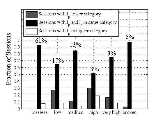
Figure 6 shows the
fraction of sessions in each category (the number at the top of each
group). About 78% of the sessions are classified as lossless or low
loss.
For each category we also
show, with two or three adjacent bars, the fraction of sessions for
which the loss rate estimates with Poisson and Periodic probing agree
(central bar), as well as the fraction of sessions
for which Periodic probing leads to a lower (left bar) or higher
(right bar) category. Notice that the two probing techniques agree in
more than 70%
of the sessions.
Given that the loss process in a congested link can be highly bursty,
and since our sample size is rather small to accurately
estimate low loss rates,
it is not surprising that about 10-30% of the sessions observe
different loss categories with Poisson and Periodic
probing.
Figure 6:
Classification of loss rate estimates in six categories.
|
|
5 Packet pair dispersion measurements
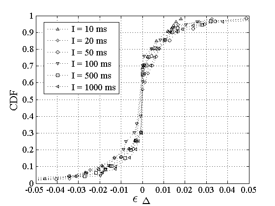
Figure 7:
The relative difference  between Poisson and Periodic dispersion
medians. between Poisson and Periodic dispersion
medians.
|
|
Comparison of median dispersions:
In the dispersion measurements, we send back-to-back packet pairs
of size from the source to the destination.
The latter measures the time spacing (``dispersion'')  between the
arrival of the first and the second packet.
The dispersion at the destination is related to the cross
traffic load and available bandwidth in the network path
[4].
Specifically, the higher the cross traffic load is at the path's
bottleneck, the wider the dispersion of the packet pairs at the
destination
due to the interference of cross traffic between the probing pair. between the
arrival of the first and the second packet.
The dispersion at the destination is related to the cross
traffic load and available bandwidth in the network path
[4].
Specifically, the higher the cross traffic load is at the path's
bottleneck, the wider the dispersion of the packet pairs at the
destination
due to the interference of cross traffic between the probing pair.
For these measurements, if one of the two packets is lost, the
corresponding pair is ignored.
Note that the average probing interarrival controls
the time spacing between successive packet pairs, not between packets
of the same pair, which are always sent back-to-back.
Let  and and  be the median
dispersions estimated from the Poisson and Periodic probing streams,
respectively, for a particular session.
We define the relative difference between the two dispersion
medians as be the median
dispersions estimated from the Poisson and Periodic probing streams,
respectively, for a particular session.
We define the relative difference between the two dispersion
medians as
 . Figure 7 shows the empirical CDF of . Note that about 90% of the sessions have . Figure 7 shows the empirical CDF of . Note that about 90% of the sessions have  2.5%,
while the relative difference does not exceed 8%.
Consequently, as in the case of RTTs, we see that the Poisson
and Periodic probing processes estimate practically the same dispersion,
at least in terms of a point estimate for the first moment. 2.5%,
while the relative difference does not exceed 8%.
Consequently, as in the case of RTTs, we see that the Poisson
and Periodic probing processes estimate practically the same dispersion,
at least in terms of a point estimate for the first moment.
Goodness-of-fit test: We also examined whether the two
probing processes observe the
same dispersion distribution.
To do so, we used again the KL test described in § 3.
This time the null hypothesis is that the two
dispersion
samples (Poisson and Periodic) for a given session follow an
identical distribution.
Figure 8:
Distribution of P-values for the null hypothesis ,
applied to dispersion sessions.
|
|
Figure 8 shows the
distribution of P-values
reported by the KL test, for various probing interarrivals .
Notice that the P-value is less than 10% for only
5-10% of the sessions.
The rest of the sessions have significantly higher P-values,
implying that we can assume to be true.
6 Discussion
The experimental results in this paper indicate that there
may not be a significant difference between Poisson
and Periodic probing, at least in the context of real Internet
measurements. This does not mean that we recommend
the use of Periodic probing over Poisson probing. We note however
that measurement studies that use, or
have used, Periodic probing should not be dismissed based
on that fact, and they may also have practical benefits compared to
Poisson probing.
A few additional remarks on the accuracy of Poisson
and Periodic probing follow.
First, it is important to note that the fraction of dropped Poisson
probing packets
at a network queue does not estimate the packet loss rate,
i.e., the fraction of dropped packets among all arrived
packets;
instead, it estimates the fraction of time that the queue is full.
The latter is equal to the loss rate in a queue with Poisson packet
arrivals;
this follows applying the PASTA property to all packets (not only the
probing packets).
For more bursty traffic, however, the packet loss rate can be higher
than
the fraction of time that the queue is full.
Consequently, even if Poisson and Periodic probing
observe the same loss rate, that fraction should
not be expected to be equal to the underlying loss rate.
Second, Periodic probing at a certain interarrival
cannot "see" effects that occur in lower time scales
(or higher frequency).
In the case of loss rate estimation, in particular,
loss events in Drop-Tail queues can be very bursty.
If the duration of loss bursts is much lower than ,
then Periodic probing may underestimate both the full-queue
probability and the loss rate. Poisson probing, however, with a
sufficiently
large number of samples, should be able to estimate the full-queue
probability.
Third, it is important to note that even if
we generate a Poisson probing stream at the source, the
probing packets may not arrive at the bottleneck
link as a Poisson process. Consider, for instance,
that the output of an  queue is not a Poisson
process. In more practical terms, if the probing
packets go through a store-and-forward link with
capacity queue is not a Poisson
process. In more practical terms, if the probing
packets go through a store-and-forward link with
capacity  , then their interarrivals after that link
cannot be lower than , then their interarrivals after that link
cannot be lower than  , where is the
packet size.
Consequently, the probing packets will no longer be a Poisson stream
and PASTA will not apply. This issue is important for Internet
measurements,
given that most network paths go through multiple queues. , where is the
packet size.
Consequently, the probing packets will no longer be a Poisson stream
and PASTA will not apply. This issue is important for Internet
measurements,
given that most network paths go through multiple queues.
Appendix: Density estimation
Suppose that we are given two samples  and and  that take values in a range
  . We want to
approximate the probability density functions
of the two samples
with the probability mass functions . We want to
approximate the probability density functions
of the two samples
with the probability mass functions  and and  defined over a set of bins , such that
and is the fraction of
measurements in the defined over a set of bins , such that
and is the fraction of
measurements in the  bin
from and , respectively, and bin
from and , respectively, and
 = =
 =1.
We select the initial bin size =1.
We select the initial bin size  based on the
Freedman-Diaconis rule as based on the
Freedman-Diaconis rule as
 ,
where ,
where  is the number of samples in the joint sample is the number of samples in the joint sample  and
and  is the interquartile range of [10].
We then proceed to determine the bin boundaries, with the first
bin placed based on the minimum measurement, and to estimate the
functions and . is the interquartile range of [10].
We then proceed to determine the bin boundaries, with the first
bin placed based on the minimum measurement, and to estimate the
functions and .
The problem, however, is that some bins may not include enough
measurements from each sample.
When that is the case we are not able to accurately estimate
the ``likelihood ratio''  of Equation 2. To guarantee that each bin
contains at least a certain number
of measurements from both samples, we use an adaptive histogram
approach. Specifically, if a bin does not include at least
1% of the measurements from each sample, we merge that
bin with the bin at its right. The process is repeated until the
previous constraint is met. If there are no measurements from that
sample at any of the right bins,
we merge the problematic bin with the bin at its left. In practice, we
found that the previous heuristic is quite
robust, as long as the two samples take values over approximately
the same range. of Equation 2. To guarantee that each bin
contains at least a certain number
of measurements from both samples, we use an adaptive histogram
approach. Specifically, if a bin does not include at least
1% of the measurements from each sample, we merge that
bin with the bin at its right. The process is repeated until the
previous constraint is met. If there are no measurements from that
sample at any of the right bins,
we merge the problematic bin with the bin at its left. In practice, we
found that the previous heuristic is quite
robust, as long as the two samples take values over approximately
the same range.
We are grateful to Prof. Paul Kvam (ISYE, Georgia Tech)
for suggesting the use of relative entropy in a goodness-of-fit test.
This work was supported in part by the NSF
CAREER award ANIR-0347374, NSF award ANI-024085, and by a gift from
DoCoMo USA Labs.
-
- 1
- V. Paxson, G.Almes, J.Madhavi, and M.Mathis,
Framework for IP Performance Metrics, May 1998,
RFC 2330.
- 2
- V. Paxson,
Measurements and Analysis of End-to-End Internet Dynamics,
Ph.D. thesis, University of California, Berkeley, Apr. 1997.
- 3
- Y. Zhang, N. Duffield, V. Paxson, and
S. Shenker,
``On the Constancy of Internet Path Properties,''
in Proceedings of ACM/USENIX Internet Measurement Workshop (IMW),
Nov. 2001, pp. 197-211.
- 4
- J. Strauss, D. Katabi, and F. Kaashoek,
``A Measurement Study of Available Bandwidth Estimation Tools,''
in Proceedings of ACM/USENIX Internet Measurement Conference (IMC),
2003.
- 5
- D. Papagiannaki, S. Moon, C. Fraleigh,
P. Thiran, F. Tobagi, and C. Diot,
``Analysis of Measured Single-Hop Delay from an Operational Backbone
Network,''
in Proceedings of IEEE INFOCOM, 2002.
- 6
- R. Caceres, N. G. Duffield, J. Horowitz, and
D. Towsley,
``Multicast-Based Inference of Network-Internal Loss Characteristics,''
IEEE Transactions in Information Theory, pp. 2462-2480,
1999.
- 7
- R. Wolff,
``Poisson Arrivals See Time Averages,''
Operations Research, vol. 30, no. 2, pp. 223-231, 1982.
- 8
- J. Sommers, P. Barford, N. G. Duffield, and
A. Ron,
``Improving Accuracy in End-to-End Packet Loss Measurements,''
in Proceedings ACM SIGCOMM, Aug. 2005.
- 9
- M. Lexa,
``Useful Facts about the Kullback-Leibler Discrimination Distance,''
Tech. Rep., Rice University, 2004.
- 10
- D. Scott,
Multivariate Density Estimation: Theory, Practice and
Visualization,
Prentice Hall, 1992.
------------------------------------------------------------------------------------------------------------------------------
Poisson versus periodic path probing (or, does PASTA matter?)
This document was generated using the
LaTeX2HTML
translator Version 2002 (1.62), and later edited manually.
Copyright © 1993, 1994, 1995, 1996,
Nikos Drakos,
Computer Based Learning Unit, University of Leeds.
Copyright © 1997, 1998, 1999,
Ross Moore,
Mathematics Department, Macquarie University, Sydney.
The translation was initiated by Muhammad Mukarram Bin Tariq on
2005-08-10
  
Muhammad Mukarram Bin Tariq
2005-08-10
|