Accuracy of core flow slicing algorithm

In this section, we evaluate the core flow slicing algorithm against the ``full-state'' approach. These experiments provide more insight into the efficacy of the flow slicing algorithm and the effect of changing various variables such as flow slicing probability and slice length on the memory usage and the mean relative error of results.

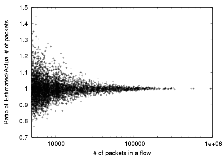
Figure 2: Scatter plot depicting the accuracy of packet count estimates based on flow slices.

Are estimates unbiased? For this experiment, we fix the flow slicing probability $p$ to 0.8% (1 in 125) and the slice duration to 60 seconds. Figure 2 shows the scatter plot of ratio of the estimated and true flow sizes (in number of packets) on the y-axis with increasing true flow size on the x-axis. Note that the plot only shows flows that have more than 5,000 packets throughout the duration of the trace (1 hour). From this scatter plot, we can see that most of the flows have been accurately estimated (within 10%). The estimates converge to the true values as the flow size increases. The presence of two-sided errors empirically confirms the unbiasedness of estimates based on flow slicing.

Figure 3: Trade-off between the mean relative error and memory usage as we increase flow slicing probability.

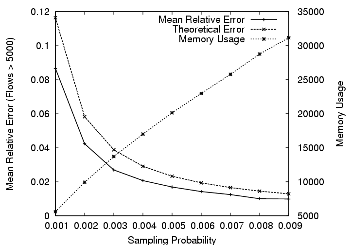What is the effect of flow slicing probability on the accuracy of these estimates ? According to , increasing flow slicing probability increases the accuracy of estimated flow sizes. Besides, the memory usage should increase as the slicing probability increases. In Figure 6.1, the mean relative error for flows larger than 5,000 and the corresponding memory usage have been plotted with varying slicing probability on the x-axis. Apart from the empirical value of the mean relative error, we also plot the theoretical value based on . Figure 6.1 confirms that increasing slicing probability decreases the mean relative error while increasing the memory usage. It can also be observed from the figure that the theoretical and empirical values of mean relative errors are in close agreement thus validating the analysis in .

Figure: Scatter plot depicting the errors introduced in interpolating bin measures from slices.

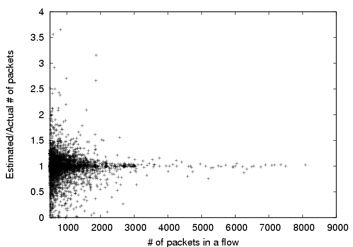What kinds of errors do we introduce by interpolating the number of packets in time bins? The goal of this experiment is to study the errors introduced when interpolating the number of packets in various time bins from flow slices that do not use bins (they only store the timestamps of the first and last packet). In , the y-axis has the ratio of estimated to actual size of the flow in a given bin and the x-axis has the actual flow size (in packets). For this experiment, we used a slice length of 90 seconds and divided it up equally into 10 bins of size 9 seconds each. Two conclusions can be drawn from the results in . First, for large flows, the error in the estimates obtained by interpolating bins from slices is insignificant. On the other hand, for relatively small flows, interpolating from flow slices results in much higher error. This is because we divide the entire volume of traffic for a particular flow among the bins it covers (see for more details); the error depends on the timing of bursts of traffic. Of course, to capture the fine grained traffic information, the extension proposed in could be used, but it would result in higher memory requirements. Second, we can observe the presence two-sided errors indicates lack of bias.

Table 4: Comparison of the error introduced by multifactor smart sampling and smart sampling into estimates of traffic of various applications (average of 10 runs with different seeds). Both algorithms were configured to reduce the number of flow records from 1,700,000 to around 190,000.

Port number used as	Multifactor s. s. error			Smart sampling error			Actual traffic
aggregation key	Pkts	Bytes	SYNs	Pkts	Bytes	SYNs	Pkts	Bytes	SYNs
Web (80)	0.4%	0.7%	0.8%	0.3%	0.1%	1.6%	17.5M	1582M	1852K
Kazaa (1214)	0.4%	0.2%	2.4%	0.6%	0.1%	12.4%	2.67M	1527M	44.9K
eDonkey (4662)	0.5%	0.7%	1.5%	1.0%	0.2%	4.5%	2.96M	1075M	344K
telnet (23)	0.6%	0.8%	4.9%	0.9%	1.0%	39.2%	1.84M	79.1M	12.0K
SMB (445)	1.3%	1.6%	1.1%	2.5%	1.8%	3.1%	1.50M	93.3M	1380K
SMTP (25)	1.9%	1.0%	1.4%	2.7%	0.9%	6.4%	0.43M	130M	86.9K
DNS (53)	1.8%	2.4%	3.6%	2.7%	1.7%	16.8%	0.45M	34.8M	6.02K

What is the effect of multi-factor smartsampling on the accuracy of estimates? In , we proposed a modification to smart sampling to improve the accuracy of the estimates for the number of flow arrivals. Table 4 summarizes the results of our experiment comparing multi-factor smart sampling with smart sampling. Before we discuss the details of this experiment, we want to note that we found that , that only the first packet of a flow can have the SYN flag set, is often violated in our trace. For some applications, the average number of packets with the SYN flag set per flow is almost 2 (due to SYN retransmissions). This affects all estimators of flow arrivals based on SYN counts. In this experiment, we do not aim to evaluate the accuracy of estimators based on SYN counts, but the effect of smart sampling on their estimates. Therefore, we do not measure the error relative to the actual number of flow arrivals, but to the estimate of flow arrivals based on the input to the two smart sampling algorithms. The input we used is the result of Flow Slices with a packet sampling probability of $q=1/4$ and flow slicing probability of $p=1/4$, using a slice length of 60 seconds and an inactivity timeout of 15 seconds. The threshold used for smart sampling is $z=50,000$ bytes. The thresholds used for multi-factor smart sampling, $z_s=1,000$ packets, $z_b=500,000$ bytes and $z_a=50$ flows, have been selected so that it produces approximately same number of records as smart sampling (from 1,700,000 down to roughly 190,000). Table 4 shows the error introduced by the two variants of smart sampling into estimates of the traffic of various applications identified by destination port numbers. While smart sampling introduces very large errors in the flow arrival estimates, multi-factor smart sampling ensures that the errors are comparable to packet and byte count estimates. For example, smart sampling incurs an error of 39.2% for telnet because it's small flows (approximately 6,600 bytes per flow on average compared to 34,000 for Kazaa) are discriminated against by smart sampling. Multi-factor smart sampling, on the other hand, achieves more accurate flow arrival counts by biasing its sampling towards records with non-zero flow arrivals. This typically results in only a slight reduction in the accuracy of packet and byte count estimates.