1
Luca Parolini, Bruno Sinopoli, Bruce H. Krogh
Dept. of Electrical and Computer Engineering
Carnegie Mellon University
C.0GeneralSystem architecture[Data center, Energy management, Energy efficiency, Thermal modeling, Optimization, Optimal control, Cyber-physical systems]
Data servers account for nearly 1.5% of total electricity consumption in the U.S. at a cost of approximately $4.5 billion per year [16]. Data center peak load exceeded 7 GW in 2006, and without intervention is destined to reach 12 GW by 2011, about the power generated by 25 baseload power plants. To address this emerging problem, this paper advocates a coordinated approach to data center energy management.
In most data centers today, the cooling and the computational subsystems are controlled independently. Computer room air conditioning (CRAC) units operate at levels necessary to keep the hottest regions in the data center below critical temperature limits. Computational tasks are allocated to achieve the desired performance with server power states that minimize overall server energy consumption. Some load management strategies consider the influence of the server loads on the temperature distribution, but CRAC control remains thermostatic. Coordinating cooling and load management requires a unified modeling framework that represents the interactions of these two subsystems. We present the elements of such a framework and formulate the coordinated control problem as a constrained Markov decision process (CMDP). Simulation results for a small system illustrate the potential benefits of this approach.
The following section reviews previous work on energy management strategies in data centers. Section 3 proposes an integrated thermal and computational model. Temperature dynamics are modeled by a network of interconnected components reflecting the spatial distribution of servers, CRAC units, and non-computational components in the data center. A second network models the distribution of the computational load among the servers. The server power states influence both networks. In Sec. 4, the energy management problem is formulated as a CMDP. Decision variables include the CRAC set points, the allocation of tasks to servers, and server power states. The dynamic MDP strategy determines these control variables as a function of the system state to minimize the integral of the weighted sum of power consumption and computational performance. Section 5 presents simulation results for a simple system, comparing the optimal MDP strategy to a conventional decoupled control of the cooling and computational subsystems. The final section identifies several directions for further research.
 |
Early work on energy minimization for data centers focused on computational fluid dynamic (CFD) models to analyze and design server racks and data center configurations to optimize the delivery of cold air, and thereby minimize cooling costs [13,12]. Subsequent papers focused on the development of optimal load-balancing policies, at both the server and rack levels. Constraints on these policies were either the minimum allowed computational performance or the maximum allowed peak power consumption [5,3,4,18,6,15].
Some recent papers have considered policies to minimize the total data center energy consumption by distributing the workload in a temperature-aware manner [11,2]. Research on load distribution based on the thermal state of the data center, led to the development of fast and accurate estimation techniques to determine the temperature distribution in a data center, based on sparsely distributed temperature measurements [10,14]. Approaches to the data center energy management problem based on queueing theory and Markov decision processes can be found in [9,17].
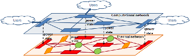
As illustrated in Fig. 1, we model a data center as two coupled networks: a computational network and a thermal network. The computational network describes the relationship between the streams of data incoming from external users and generated by the data center itself and the computational load assigned to each server. The computational network is composed of server nodes that interact through the exchange of workloads. We call jobs the computational requests that enter and leave the data center and tasks the computational requests exchanged within the data center. A single job can be broken into multiple tasks and similarly, multiple tasks can be merged into a single job. A server's workload is then defined as the number of tasks arriving at the node per unit of time. The data center networks interact with the external world by exchanging jobs at the computational network level and through the consumption of electrical power at the thermal network level.
The thermal network describes the thermal energy exchange at the
physical level of the data center and accounts for the power
consumed by the CRAC units, IT devices and non-computational
devices. The thermal network presents three types of nodes:
server, CRAC and environment nodes. Environment
nodes represent IT devices other than servers, non-computational
devices and external environmental effects (e.g. weather). Each
node in the thermal network has an input temperature
![]() [
[![]() C],
an output temperature
C],
an output temperature
![]() [
[![]() C] and an electrical power
consumption
C] and an electrical power
consumption
![]() [W]. The electrical power consumption is allowed to
be either a controlled input or an output of a node (the result of
some other controlled or uncontrolled processes).
[W]. The electrical power consumption is allowed to
be either a controlled input or an output of a node (the result of
some other controlled or uncontrolled processes).
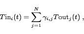
Following the thermal model proposed in
[14], we assume that the input
temperature
![]() [
[![]() C] of a node
C] of a node ![]() is given by a convex
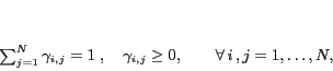
linear combination of the output temperatures of all other nodes and the value of each coefficient
is given by a convex
linear combination of the output temperatures of all other nodes and the value of each coefficient ![]() depends upon the particular data center
layout:
depends upon the particular data center
layout:
We model the computational server node as a G/M/1 queue. The task
inter-arrival distribution is given by a combination of the
inter-arrival jobs at the data center and server interaction in the
computational network, while the service time is exponentially
distributed with parameter ![]() . Measurements taken on a server in our laboratory, shown in
Fig. 2, show that the thermal part of server node can
be modeled as a first-order linear time-invariant (LTI) system
defined by the following differential equation:
. Measurements taken on a server in our laboratory, shown in
Fig. 2, show that the thermal part of server node can
be modeled as a first-order linear time-invariant (LTI) system
defined by the following differential equation:
 |
A server node can represent either a single server or a set of servers. In the second case it is necessary to identify aggregate definitions of the node power state, power consumption, input and output temperatures.
For the sake of clarity, we show how to formulate the data center energy
management problem as a finite CMDP using a particular instantiation
of the data center model. Generalization to an arbitrary case is
straightforward, but would require the introduction of more
notation. Here we assume that the data center is composed of ![]() server nodes,
server nodes, ![]() CRAC nodes and
CRAC nodes and ![]() environment nodes. Also, we
will consider a discrete-time model of the data center with time
step
environment nodes. Also, we
will consider a discrete-time model of the data center with time
step
![]() .
.
In order to formulate our optimization problem as a finite CMDP we have to
identify: a finite set ![]() of states, a finite set
of states, a finite set ![]() of
actions from which the controller can choose at each step
of
actions from which the controller can choose at each step
![]() , a set
, a set ![]() of transition
probabilities representing the probability of moving from a state
of transition
probabilities representing the probability of moving from a state
![]() to a state
to a state ![]() when the action
when the action ![]() is applied, and a function
is applied, and a function
![]() of immediate costs for
each time step.
The total cost over a given time horizon is the sum of the cost incurred at each time step.
of immediate costs for
each time step.
The total cost over a given time horizon is the sum of the cost incurred at each time step.
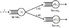
For this example, we assume jobs arrive only through the third server node, called the scheduler, and there is no workload exchange between server nodes one and two, as illustrated in Fig. 3.
Jobs arrive at the scheduler one at a time at the beginning of every time slot ![]() and the arrival events are i.i.d. Bernoulli random variables of parameter
and the arrival events are i.i.d. Bernoulli random variables of parameter ![]() . The execution time of each job is independent from the execution time of all other jobs. During a single time slot a job is received by the scheduler and it is sent to one of the server nodes during the same time slot, according to a Bernoulli distributed random variable
. The execution time of each job is independent from the execution time of all other jobs. During a single time slot a job is received by the scheduler and it is sent to one of the server nodes during the same time slot, according to a Bernoulli distributed random variable ![]() . If
. If ![]() the job is sent to the server node
the job is sent to the server node ![]() , while if
, while if ![]() the job is sent to the server node
the job is sent to the server node ![]() . The mean
value of
. The mean
value of ![]() can be chosen from a finite set of values.
can be chosen from a finite set of values.
In this example, there are no differences between jobs and tasks and the controller action on the computational network workload exchange reduces to the choice of the mean value of ![]() .
.
The scheduler does not participate in thermal energy exchange between server nodes and CRAC node and its power consumption
![]() is
identically null for all of its power states. In the rest of the paper then, we will neglect its presence.
is
identically null for all of its power states. In the rest of the paper then, we will neglect its presence.
CRAC node is assumed to have no dynamics and hence, its output temperature coincides with
![]() when
when
![]() , while it is equal to
, while it is equal to
![]() when
when
![]() .
.
In order to reach the goal of a finite set of states we have to
discretize the set of admissible values for
![]() ,
,
![]() and
and
![]() . We define
. We define
![]() as the quantized version
of
as the quantized version
of
![]() and similarly for
and similarly for
![]() . States of the CMDP will then be given by the pairs
. States of the CMDP will then be given by the pairs
![]() , while actions will be given by tuple
, while actions will be given by tuple
![]() .
.
We model the uncertainty on
![]() as a random variable uniformly distributed in
as a random variable uniformly distributed in
![]() .
.
![]() and
and
![]() represent
respectively the minimum and the maximum temperature values allowed
for
represent
respectively the minimum and the maximum temperature values allowed
for
![]() when its discretized version has value
when its discretized version has value
![]() , while
, while
![]() represents the value of
represents the value of
![]() associated with the state
associated with the state
![]() . The uncertainty about the true
values of
. The uncertainty about the true
values of
![]() and
and
![]() determines each entry of
determines each entry of
![]() .
.
The selected cost function is:
 |
(4) |
Another constraint we add imposes that each server node has to be set to its most conservative power state if no tasks will be sent to it and that its mean task execution rate has to be greater than or equal to its task arrival rate.
This particular cost function can be called a discounted energy![[*]](footnote.png) cost since we are weighting the energy spent at the present time more than the one that will be spent in the far future.
cost since we are weighting the energy spent at the present time more than the one that will be spent in the far future.
We compare our control algorithm against a typical hierarchical greedy scheduling algorithm that first chooses the best values for ![]() ,
, ![]() and
and ![]() to minimize the cost function given in equation (6) and then it selects the best value for
to minimize the cost function given in equation (6) and then it selects the best value for
![]() in order to minimize the power consumption of the CRAC node enforcing the thermal constraints. The performances of the two algorithms are tested against four different job arrival rates:
in order to minimize the power consumption of the CRAC node enforcing the thermal constraints. The performances of the two algorithms are tested against four different job arrival rates:
![]() .
.
In this simulation we assume that server node 1 consumes more power than server node 2 for the same value of the task execution rate, while its thermal effect on the input temperature of the CRAC node is reduced with respect to the effects of server node 2. Finally we assume that the power consumption of the data center is mainly driven by the power of the CRAC node.
 |
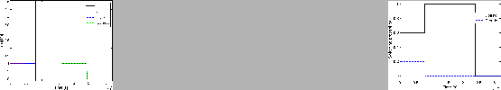 |
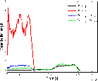
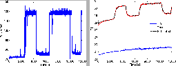
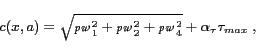
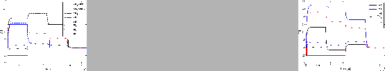
As shown in Fig. 4(a) and 4(b), using mainly server node one instead of the more power efficient server node two, the optimal controller is able to maintain a smaller difference between the input and output temperature of the CRAC node if compared to the greedy controller. Hence, as shown in Fig. 7(a), the optimal controller reaches a lower data center power consumption profile than the greedy controller and consequently a lower overall energy consumption, Fig. 7(b). As depicted in Fig. 6 energy minimization is obtained without heavily affecting the computational characteristics of the data center.
There are several directions for further research. The CMDP formulation will be intractable for detailed models of real systems due to the exponential growth of the state space. This problem can be addressed by using hierarchical models. In our modeling framework, the nodes in each network can represent aggregate sets of devices, each of which can be modeled by lower-level thermal and computational networks. We are currently developing the details of such hierarchical models. Hierarchical models will lead naturally to hierarchical and distributed control strategies. Initial steps in this direction can be found in [15].
 |
Another issue regards the modeling and allocation of jobs and tasks in the computational network. Our current model assumes homogeneous and independent tasks and simple FIFO tasks queues at each server. In real systems, there can be a complex mixture of tasks and servers work on more than one task at a time. There may also be dynamic exchanges and reallocation of tasks that are in progress. We are currently investigating methods for incorporating and exploiting these features.
Finally, our model has several parameters that need to be determined for specific applications. This requires the development of effective system identification algorithms, which need to be implemented on line since the parameter values can be time varying.
This document was generated using the LaTeX2HTML translator Version 2002-2-1 (1.70)
Copyright © 1993, 1994, 1995, 1996,
Nikos Drakos,
Computer Based Learning Unit, University of Leeds.
Copyright © 1997, 1998, 1999,
Ross Moore,
Mathematics Department, Macquarie University, Sydney.
![\begin{displaymath}
J(\mathbf{p},\mathbf{{T\textrm{ref}}},\mathbf{s},\alpha_\tau...
...lpha)\sum_{i=1}^\infty\alpha^i\mathsf{E}\Big[c(x(i),a(i))\Big],\end{displaymath}](img76.png)