5th USENIX Conference on File and Storage Technologies - Paper
Pp. 1–16 of the Proceedings
Disk failures in the real world:
What does an MTTF of 1,000,000 hours mean to you?
Bianca Schroeder Garth A. Gibson
Computer Science Department
Carnegie Mellon University
{bianca, garth}@cs.cmu.edu
Component failure in large-scale IT installations
is becoming an ever larger problem as the number of
components in a single cluster approaches a million.
In this paper, we present and analyze field-gathered disk replacement data from a number
of large production systems, including high-performance computing sites and
internet services sites.
About 100,000 disks are covered by this data, some
for an entire lifetime of five years. The data include drives
with SCSI and FC, as well as SATA interfaces.
The mean time to failure (MTTF) of those drives, as specified in their datasheets,
ranges from 1,000,000 to 1,500,000 hours, suggesting a nominal annual failure rate of at most
0.88%.
We find that in the field, annual disk replacement rates typically exceed 1%, with 2-4%
common and up to 13% observed on some systems. This
suggests that field replacement is a fairly different process than one might
predict based on datasheet MTTF.
We also find evidence, based on records of disk replacements in the field, that failure rate is not constant with age,
and that, rather than a significant infant mortality effect,
we see a significant early onset of wear-out degradation. That is,
replacement rates in our data grew constantly with age, an
effect often assumed not to set in until after a nominal lifetime of 5 years.
Interestingly, we observe little difference in replacement rates
between SCSI, FC and SATA drives, potentially an indication that
disk-independent factors, such as operating
conditions, affect replacement rates more than
component specific factors. On the other hand, we see only one instance
of a customer rejecting an entire population of disks as a bad batch, in this
case because of media error rates, and this instance involved SATA disks.
Time between replacement,
a proxy for time between failure,
is not well modeled by an exponential distribution
and exhibits significant levels of correlation, including
autocorrelation and long-range dependence.
Despite major efforts, both in industry and in academia,
high reliability remains a major challenge in running large-scale IT systems,
and disaster prevention and cost of actual disasters
make up a large fraction of the total cost of ownership. With ever larger server clusters, maintaining high levels of reliability and availability is a growing
problem for many sites, including high-performance computing systems and internet
service providers.
A particularly big concern is the reliability of storage systems, for several
reasons.
First, failure of storage can not only cause temporary data unavailability, but
in the worst case it can lead to permanent data loss. Second, technology
trends and market forces may combine to make storage system failures occur
more frequently in the future [24]. Finally, the size of storage systems in modern,
large-scale IT installations has grown to an unprecedented scale with thousands of
storage devices, making component failures the norm rather than the exception [7].
Large-scale IT systems,
therefore, need better system design and management
to cope with more frequent failures.
One might expect increasing levels of redundancy
designed for specific failure modes [3,7], for example. Such designs
and management systems are based on very simple models of component failure and repair processes [22].
Better knowledge about the statistical
properties of storage failure processes, such as the distribution of time between failures,
may empower researchers and designers to develop new, more reliable and available storage systems.
Unfortunately, many aspects of disk failures in real systems are not well understood,
probably because the owners of such systems are reluctant to release failure data or do
not gather such data.
As a result, practitioners usually rely on vendor specified parameters, such as mean-time-to-failure (MTTF),
to model failure processes, although many are skeptical of the accuracy of
those models [4,5,33].
Too much academic and corporate research is based on anecdotes and back of
the envelope calculations, rather than empirical data [28].
The work in this paper is part of a broader research agenda with the long-term goal of
providing a better understanding of failures in IT systems by collecting,
analyzing and making publicly available a diverse set of real failure histories
from large-scale production systems.
In our pursuit, we have spoken to a number of large production sites and were
able to convince several of them to provide failure data from some of their systems.
In this paper, we provide an analysis of seven data sets we have collected, with a focus
on storage-related failures. The data sets come from a number of large-scale
production systems, including high-performance computing sites
and large internet services sites, and consist primarily of hardware replacement logs.
The data sets vary in duration from one month to five years
and cover in total a population of more than 100,000 drives
from at least four different vendors. Disks covered by this data include
drives with SCSI and FC interfaces, commonly
represented as the most reliable types of disk drives, as well as drives with SATA interfaces, common
in desktop and nearline systems.
Although 100,000 drives is a very large sample relative to previously published studies, it
is small compared to the estimated 35 million enterprise drives, and 300 million total
drives built in 2006 [1]. Phenomena such as bad batches caused by fabrication line changes
may require much larger data sets to fully characterize.
We analyze three different aspects of the data.
We begin in Section 3 by asking how disk replacement frequencies
compare to replacement frequencies of other hardware components.
In Section 4, we provide a quantitative analysis of disk replacement rates
observed in the field and compare our observations with common predictors
and models used by vendors.
In Section 5, we analyze the statistical properties of
disk replacement rates. We study correlations between disk replacements and identify the key
properties of the empirical distribution of time between replacements,
and compare our results to common models and assumptions.
Section 6 provides an overview of related work and Section 7 concludes.
Table 1:
Overview of the seven failure data sets. Note that the disk count given in the table is the
number of drives in the system at the end of the data collection period. For some systems the number
of drives changed during the data collection period, and we account for that in our analysis.
The disk parameters 10K and 15K refer to the rotation speed in revolutions per minute;
drives not labeled 10K or 15K probably have a rotation speed of 7200 rpm.
|
Data set |
Type of |
Duration |
#Disk |
# Servers |
Disk |
Disk |
MTTF |
Date of first |
ARR |
|
|
cluster |
|
events |
|
Count |
Parameters |
(Mhours) |
Deploym. |
(%) |
|
HPC1 |
HPC |
08/01 - 05/06 |
474 |
765 |
2,318 |
18GB 10K SCSI |
 |
08/01 |
4.0 |
|
" |
" |
" |
124 |
64 |
1,088 |
36GB 10K SCSI |
|
" |
2.2 |
|
HPC2 |
HPC |
01/04 - 07/06 |
14 |
256 |
520 |
36GB 10K SCSI |
|
12/01 |
1.1 |
|
HPC3 |
HPC |
12/05 - 11/06 |
103 |
1,532 |
3,064 |
146GB 15K SCSI |
1.5 |
08/05 |
3.7 |
|
" |
HPC |
12/05 - 11/06 |
4 |
N/A |
144 |
73GB 15K SCSI |
1.5 |
" |
3.0 |
|
" |
HPC |
12/05 - 08/06 |
253 |
N/A |
11,000 |
250GB 7.2K SATA |
1.0 |
" |
3.3 |
|
HPC4 |
Various |
09/03 - 08/06 |
269 |
N/A |
8,430 |
250GB SATA |
 |
09/03 |
2.2 |
|
" |
HPC |
11/05 - 08/06 |
7 |
N/A |
2,030 |
500GB SATA |
|
11/05 |
0.5 |
|
" |
clusters |
09/05 - 08/06 |
9 |
N/A |
3,158 |
400GB SATA |
|
09/05 |
0.8 |
|
COM1 |
Int. serv. |
May 2006 |
84 |
N/A |
26,734 |
10K SCSI |
|
2001 |
2.8 |
|
COM2 |
Int. serv. |
09/04 - 04/06 |
506 |
9,232 |
39,039 |
15K SCSI |
|
2004 |
3.1 |
|
COM3 |
Int. serv. |
01/05 - 12/05 |
2 |
N/A |
56 |
10K FC |
|
N/A |
3.6 |
|
" |
" |
" |
132 |
N/A |
2,450 |
10K FC |
|
N/A |
5.4 |
|
" |
" |
" |
108 |
N/A |
796 |
10K FC |
|
N/A |
13.6 |
|
" |
" |
" |
104 |
N/A |
432 |
10K FC |
|
1998 |
24.1 |
|
2 Methodology
2.1 What is a disk failure?
While it is often assumed that disk failures follow a simple fail-stop model (where disks either work perfectly or
fail absolutely and in an easily detectable manner [22,24]), disk failures are much more complex in reality.
For example, disk drives can experience latent sector faults or transient performance problems. Often it is hard
to correctly attribute the root cause of a problem to a particular hardware component.
Our work is based on hardware replacement records and logs, i.e. we focus on disk conditions that lead a drive customer to treat
a disk as permanently failed and to replace it.
We analyze records from a number of large production systems, which contain a record
for every disk that was replaced in the system during the time of the data collection.
To interpret the results of our work correctly it is crucial to understand the process of how this data was created.
After a disk drive is identified as the likely culprit in a problem, the operations staff (or the computer system itself)
perform a series of tests on the drive to assess its behavior. If the behavior qualifies as faulty according to the customer's definition,
the disk is replaced and a corresponding entry is made in the hardware replacement log.
The important thing to note is that there is not one unique definition for when a drive is faulty.
In particular, customers and vendors might use different definitions.
For example, a common way for a customer to test a drive is to read all of its sectors to see if any reads experience problems,
and decide that it is faulty if any one operation takes longer than a certain threshold.
The outcome of such a test will depend on how the thresholds are chosen.
Many sites follow a ``better safe than sorry'' mentality, and use even more rigorous testing.
As a result, it cannot be ruled out that a customer may declare a disk faulty,
while its manufacturer sees it as healthy.
This also means that the definition of ``faulty'' that a drive customer uses does not necessarily
fit the definition that a drive manufacturer uses to make drive reliability projections.
In fact, a disk vendor has reported that for 43% of all disks returned by customers they find no problem with the disk [1].
It is also important to note that the failure behavior of a drive depends on the operating conditions, and not only on component level factors.
For example, failure rates are affected by environmental factors, such as temperature and humidity,
data center handling procedures, workloads and ``duty cycles'' or powered-on hours patterns.
We would also like to point out that the failure behavior of
disk drives, even if they are of the same model, can differ, since
disks are manufactured using processes and parts that may change. These changes,
such as a change in a drive's firmware or a hardware component or even the assembly line on which a drive
was manufactured, can change the failure behavior of a drive.
This effect is often called the effect of batches or vintage.
A bad batch can lead to unusually high drive failure rates or unusually high rates of media errors.
For example, in the HPC3 data set (Table 1) the customer had 11,000 SATA drives
replaced in Oct. 2006 after observing a high frequency of media errors during writes. Although
it took a year to resolve, the customer and vendor agreed that these drives did not meet warranty conditions.
The cause was attributed to the breakdown of a lubricant leading to unacceptably high head flying heights.
In the data, the replacements of these drives are not recorded as failures.
In our analysis we do not further study the effect of batches.
We report on the field experience, in terms of disk replacement rates, of a set of drive customers.
Customers usually do not have the information necessary to determine which of the drives they are using
come from the same or different batches.
Since our data spans a large number of drives (more than 100,000)
and comes from a diverse set of customers and systems, we assume
it also covers a diverse set of vendors, models and batches. We
therefore deem it unlikely that our results are significantly skewed by ``bad batches''.
However, we caution the reader not to assume all drives behave identically.
2.2 Specifying disk reliability and failure frequency
Drive manufacturers specify the reliability of their products in terms of two related metrics:
the annualized failure rate (AFR), which is the percentage of disk drives in a population
that fail in a test scaled to a per year estimation; and the mean time to failure (MTTF).
The AFR of a new product is typically estimated based on accelerated life and stress tests
or based on field data
from earlier products [2]. The MTTF is estimated as the number of power on hours
per year divided by the AFR. A common assumption for drives in servers is that they are powered on 100% of
the time. Our data set providers all believe that their disks are powered on and in use at all times.
The MTTFs specified for today's highest quality disks range from 1,000,000 hours to 1,500,000 hours,
corresponding to AFRs of 0.58% to 0.88%.
The AFR and MTTF estimates of the manufacturer are included in a drive's datasheet and
we refer to them in the remainder as the datasheet AFR and the datasheet MTTF.
In contrast, in our data analysis we will report the annual replacement rate (ARR) to reflect the fact
that, strictly speaking, disk replacements that are reported in the customer logs do not necessarily equal disk failures
(as explained in Section 2.1).
Table 1 provides an overview of the seven data sets used in this study.
Data sets HPC1, HPC2 and HPC3 were collected in three large cluster systems at three different
organizations using supercomputers.
Data set HPC4 was collected on dozens of independently managed HPC sites, including supercomputing sites
as well as commercial HPC sites.
Data sets COM1, COM2, and COM3 were collected in at least three different cluster systems at a large
internet service provider with many distributed and separately managed sites.
In all cases, our data reports on only
a portion of the computing systems run by each organization, as decided and selected by our sources.
It is important to note that for some systems the number
of drives in the system changed significantly during the data collection period. While the table provides only the disk count at
the end of the data collection period, our analysis in the remainder of the paper accounts for the actual date of these changes
in the number of drives.
Second, some logs also record events other than replacements, hence the number of
disk events given in the table is not necessarily equal to the number of replacements or failures. The ARR values for
the data sets can therefore not be directly computed from Table 1.
Below we describe each data set and the environment it comes from
in more detail.
HPC1 is a five year log of hardware replacements collected from a 765 node
high-performance computing cluster. Each of the 765 nodes is a 4-way SMP with 4 GB of memory
and three to four 18GB 10K rpm SCSI drives. Of these nodes, 64 are used as filesystem nodes
containing, in addition to the three to four 18GB drives, 17 36GB 10K rpm SCSI drives.
The applications running on this system are typically large-scale scientific simulations
or visualization applications.
The data contains, for each hardware replacement that was recorded during the five year lifetime of this system,
when the problem started, which node and which hardware component was affected,
and a brief description of the corrective action.
HPC2 is a record of disk replacements observed on the compute nodes of a 256 node HPC cluster.
Each node is a 4-way SMP with 16 GB of memory and contains two 36GB 10K rpm SCSI drives,
except for eight of the nodes, which contain eight 36GB 10K rpm SCSI drives each.
The applications running on this system are typically large-scale scientific simulations
or visualization applications. For each disk replacement, the data set records the number of the affected node,
the start time of the problem, and the slot number of the replaced drive.
HPC3 is a record of disk replacements observed on a 1,532 node HPC cluster.
Each node is equipped with eight CPUs and 32GB of memory. Each node, except for four login nodes,
has two 146GB 15K rpm SCSI disks.
In addition, 11,000 7200 rpm 250GB SATA drives are used in an external shared
filesystem and 144 73GB 15K rpm SCSI drives are used for the filesystem metadata.
The applications running on this system are typically large-scale scientific simulations
or visualization applications. For each disk replacement, the data set records the day of the replacement.
The HPC4 data set is a warranty service log of disk replacements. It covers three types of SATA drives
used in dozens of separately managed HPC clusters. For the first type of drive, the data spans three years,
for the other two types it spans a little less than a year. The data records, for each of the 13,618 drives,
when it was first shipped and when (if ever) it was replaced in the field.
COM1 is a log of hardware failures recorded by an internet service provider and drawing from multiple distributed sites.
Each record in the data
contains a timestamp of when the failure was repaired,
information on the failure symptoms, and a list of steps that were
taken to diagnose and repair the problem. The data does
not contain information on when each failure actually happened, only
when repair took place. The data covers a population of 26,734 10K rpm
SCSI disk drives. The total number of servers in the monitored sites is not known.
COM2 is a warranty service log of hardware failures recorded on behalf of an internet service provider
aggregating events in multiple distributed sites.
Each failure record contains a repair code (e.g. ``Replace hard drive'') and the time when
the repair was finished. Again there is no information on the start time of each failure.
The log does not contain entries for failures of disks that were replaced in the customer site by hot-swapping in a spare disk,
since the data was created by the warranty processing, which does not participate in on-site hot-swap replacements.
To account for the missing disk replacements we obtained numbers for the periodic replenishments of on-site spare disks
from the internet service provider.
The size of the underlying system changed significantly
during the measurement period, starting with
420 servers in 2004 and ending with 9,232 servers in 2006. We obtained quarterly hardware purchase records
covering this time period to estimate the size of the disk population in our ARR analysis.
The COM3 data set comes from a large external storage system used by an internet service provider and
comprises four populations of different types of FC disks (see Table 1).
While this data was gathered in 2005, the system has some legacy
components that were as old as from 1998 and were known to have been physically moved after initial installation.
We did not include these ``obsolete'' disk replacements in our analysis.
COM3 differs from the other data sets in that it
provides only aggregate statistics of disk failures, rather than individual records
for each failure. The data contains the counts of disks that failed
and were replaced in 2005 for each of the four disk populations.
2.4 Statistical methods
We characterize an empirical distribution using two import metrics:
the mean and the
squared coefficient of variation ( ). The squared coefficient of variation
is a measure of the variability of a distribution and
is defined as the squared standard deviation divided by the squared mean.
The advantage of using the squared coefficient of variation
as a measure of variability, rather than the variance or the standard deviation, is
that it is normalized by the mean, and so allows comparison
of variability across distributions with different means. ). The squared coefficient of variation
is a measure of the variability of a distribution and
is defined as the squared standard deviation divided by the squared mean.
The advantage of using the squared coefficient of variation
as a measure of variability, rather than the variance or the standard deviation, is
that it is normalized by the mean, and so allows comparison
of variability across distributions with different means.
We also consider the empirical cumulative distribution function (CDF)
and how well it is fit by four probability distributions commonly used in
reliability theory:
the exponential distribution; the Weibull distribution;
the gamma distribution; and the lognormal distribution.
We parameterize the distributions through maximum likelihood estimation and
evaluate the goodness of fit by visual inspection, the negative log-likelihood and
the chi-square tests.
We will also discuss the hazard rate of the distribution of time between replacements.
In general, the hazard rate of a random variable  with probability distribution with probability distribution  and
cumulative distribution function and
cumulative distribution function  is defined as [25] is defined as [25]
Intuitively, if the random variable denotes the time between failures, the hazard rate  describes the
instantaneous failure rate as a function of the time since the most recently observed failure.
An important property of 's distribution is whether its hazard rate is constant (which is the case
for an exponential distribution) or increasing or decreasing. A constant hazard rate implies that the
probability of failure at a given point in time does not depend on how long it has been since
the most recent failure.
An increasing hazard rate means that the
probability of a failure increases, if the time since the last failure has been long. A decreasing
hazard rate means that the probability of a failure decreases, if the time since the last failure has
been long. describes the
instantaneous failure rate as a function of the time since the most recently observed failure.
An important property of 's distribution is whether its hazard rate is constant (which is the case
for an exponential distribution) or increasing or decreasing. A constant hazard rate implies that the
probability of failure at a given point in time does not depend on how long it has been since
the most recent failure.
An increasing hazard rate means that the
probability of a failure increases, if the time since the last failure has been long. A decreasing
hazard rate means that the probability of a failure decreases, if the time since the last failure has
been long.
The hazard rate is often studied for the distribution of lifetimes. It is important to note
that we will focus on the hazard rate of the time between disk replacements, and not the hazard
rate of disk lifetime distributions.
Since we are interested in correlations between disk failures we need
a measure for the degree of correlation. The autocorrelation function (ACF)
measures the correlation of a random variable with itself at different time
lags  . The ACF, for example, can be used to determine whether the number of failures
in one day is correlated with the number of failures observed days later.
The autocorrelation coefficient can range between 1 (high positive correlation)
and -1 (high negative correlation). A value of zero would indicate no correlation,
supporting independence of failures per day. . The ACF, for example, can be used to determine whether the number of failures
in one day is correlated with the number of failures observed days later.
The autocorrelation coefficient can range between 1 (high positive correlation)
and -1 (high negative correlation). A value of zero would indicate no correlation,
supporting independence of failures per day.
Another aspect of the failure process that we will study is long-range dependence.
Long-range dependence measures the memory of a process, in particular
how quickly the autocorrelation coefficient decays with growing lags.
The strength of the long-range dependence is quantified by the Hurst exponent.
A series exhibits long-range dependence if the Hurst exponent, H, is  .
We use the Selfis tool [14] to obtain estimates of the Hurst parameter
using five different methods: the absolute value method, the variance method, the R/S method,
the periodogram method, and the Whittle estimator. A brief
introduction to long-range dependence and a description of the Hurst parameter estimators is provided
in [15]. .
We use the Selfis tool [14] to obtain estimates of the Hurst parameter
using five different methods: the absolute value method, the variance method, the R/S method,
the periodogram method, and the Whittle estimator. A brief
introduction to long-range dependence and a description of the Hurst parameter estimators is provided
in [15].
3 Comparing disk replacement frequency with that of other hardware components
Table 3:
Relative frequency of hardware component replacements for the ten most frequently replaced components in
systems HPC1, COM1 and COM2, respectively. Abbreviations are taken directly from service data and are not known to have identical
definitions across data sets.
| HPC1 |
| Component |
% |
| Hard drive |
30.6 |
| Memory |
28.5 |
| Misc/Unk |
14.4 |
| CPU |
12.4 |
| PCI motherboard |
4.9 |
| Controller |
2.9 |
| QSW |
1.7 |
| Power supply |
1.6 |
| MLB |
1.0 |
| SCSI BP |
0.3 |
|
|
| COM1 |
| Component |
% |
| Power supply |
34.8 |
| Memory |
20.1 |
| Hard drive |
18.1 |
| Case |
11.4 |
| Fan |
8.0 |
| CPU |
2.0 |
| SCSI Board |
0.6 |
| NIC Card |
1.2 |
| LV Power Board |
0.6 |
| CPU heatsink |
0.6 |
|
|
| COM2 |
| Component |
% |
| Hard drive |
49.1 |
| Motherboard |
23.4 |
| Power supply |
10.1 |
| RAID card |
4.1 |
| Memory |
3.4 |
| SCSI cable |
2.2 |
| Fan |
2.2 |
| CPU |
2.2 |
| CD-ROM |
0.6 |
| Raid Controller |
0.6 |
|
| |
|
The reliability of a system depends on all its components, and
not just the hard drive(s). A natural question is therefore what the relative
frequency of drive failures is, compared to that of other types of hardware failures.
To answer this question we consult data sets HPC1, COM1, and COM2, since these data sets
contain records for all types of hardware replacements, not only disk replacements.
Table 3 shows, for each data set, a list of the ten most frequently replaced
hardware components and the fraction of replacements made up
by each component.
We observe that while the actual fraction of disk replacements varies across the data sets
(ranging from 20% to 50%), it makes up a
significant fraction in all three cases. In the HPC1 and COM2 data sets, disk drives are the most
commonly replaced hardware component accounting for 30% and 50% of all hardware replacements,
respectively.
In the COM1 data set, disks are a close runner-up accounting for nearly 20% of all hardware replacements.
While Table 3 suggests that disks are among the most commonly replaced hardware components,
it does not necessarily imply that disks are less reliable or have a shorter lifespan than other
hardware components. The number of disks in the systems might simply be much larger than
that of other hardware components.
In order to compare the reliability of different hardware components,
we need to normalize the number of component replacements by the component's population
size.
Unfortunately, we do not have, for any of the systems,
exact population counts of all hardware components.
However, we do have enough information in HPC1 to
estimate counts of the four most frequently replaced hardware components
(CPU, memory, disks, motherboards).
We estimate that there is a total of 3,060 CPUs, 3,060 memory dimms, and 765 motherboards,
compared to a disk population of 3,406.
Combining these numbers with the data in Table 3, we conclude that
for the HPC1 system, the rate at which in five years of use a memory dimm was replaced
is roughly comparable to that of a hard drive replacement; a CPU was about 2.5 times less often replaced
than a hard drive; and a motherboard was 50% less often
replaced than a hard drive.
Table 2:
Node outages that were attributed to hardware problems broken down by the responsible hardware component.
This includes all outages, not only those that required replacement of a hardware component.
| HPC1 |
| Component |
% |
| CPU |
44 |
| Memory |
29 |
| Hard drive |
16 |
| PCI motherboard |
9 |
| Power supply |
2 |
|
The above discussion covers only failures that required a hardware component
to be replaced. When running a large system one is often interested in any hardware failure
that causes a node outage, not only those that necessitate a hardware replacement.
We therefore obtained the HPC1 troubleshooting records
for any node outage that was attributed to a hardware problem, including problems that required
hardware replacements as well as problems that were fixed in some other way.
Table 2 gives a breakdown of all records in the troubleshooting data, broken down
by the hardware component that was identified as the root cause.
We observe that 16% of all outage records pertain to disk drives (compared to 30% in Table 3),
making it the third most common root cause reported in the data. The two most commonly reported outage root causes
are CPU and memory, with 44% and 29%, respectively.
For a complete picture, we also need to take the severity of an anomalous event into account.
A closer look at the HPC1 troubleshooting data reveals that a large number of the problems
attributed to CPU and memory failures were
triggered by parity errors, i.e. the number of errors is too large for the
embedded error correcting code to correct them.
In those cases, a simple reboot will bring the affected node back up.
On the other hand, the majority of the problems that were attributed to hard disks (around 90%) lead to a drive
replacement, which is a more expensive and time-consuming repair action.
Ideally, we would like to compare the frequency of hardware problems that we report above
with the frequency of other types of problems, such software failures, network problems, etc.
Unfortunately, we do not have this type of information for the systems in Table 1.
However, in recent work [27] we have analyzed failure data covering any type of
node outage, including those caused by hardware, software, network problems, environmental problems, or
operator mistakes. The data was collected over a period of 9 years on more than 20 HPC
clusters and contains detailed root cause information.
We found that, for most HPC systems in this data, more than 50% of all outages are
attributed to hardware problems and around 20% of all outages are attributed to software problems.
Consistently with the data in Table 2, the two most common hardware components to cause a node
outage are memory and CPU. The data of this recent study [27] is not used in this paper because
it does not contain information about storage replacements.
4 Disk replacement rates
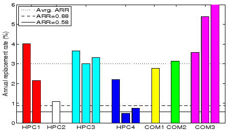
Figure 1:
Comparison of datasheet AFRs (solid and dashed line in the graph) and ARRs observed
in the field.
Each bar in the graph corresponds to one row in Table 1. The dotted line represents
the weighted average over all data sets.
Only disks within the nominal lifetime of five years are included,
i.e. there is no bar for the COM3 drives that were deployed in 1998. The third bar for COM3 in the
graph is cut off - its ARR is 13.5%.
 |
In the following, we study how field experience with disk replacements compares to
datasheet specifications of disk reliability.
Figure 1 shows the datasheet AFRs (horizontal solid and dashed line), the observed ARRs for
each of the seven data sets and the weighted average ARR for all disks less than five years old
(dotted line).
For HPC1, HPC3, HPC4 and COM3, which cover different types of disks, the graph contains several
bars, one for each type of disk, in the left-to-right order of the corresponding
top-to-bottom entries in Table 1. Since at this point we are not interested in wearout effects after the end
of a disk's nominal lifetime, we have included in Figure 1 only data for drives within their
nominal lifetime of five years. In particular, we do not include a bar for the fourth type of drives
in COM3 (see Table 1), which were deployed in 1998 and were more than seven years old at the end
of the data collection. These possibly ``obsolete'' disks experienced an ARR, during the measurement period, of 24%.
Since these drives are well outside the vendor's nominal lifetime for disks, it is not surprising
that the disks might be wearing out.
All other drives were within their nominal lifetime and are included in the figure.
Figure 1 shows a significant discrepancy between the observed ARR and the datasheet AFR for
all data sets. While the datasheet AFRs are between 0.58% and 0.88%, the observed ARRs range
from 0.5% to as high as 13.5%. That is, the observed ARRs by data set and type, are by up to a factor of 15
higher than datasheet AFRs.
Most commonly, the observed ARR values are in the 3% range.
For example, the data for HPC1, which covers almost exactly the entire nominal lifetime of five years
exhibits an ARR of 3.4% (significantly higher than the datasheet AFR
of 0.88%).
The average ARR
over all data sets (weighted by the number of drives in each data set) is 3.01%. Even
after removing all COM3 data, which exhibits the highest ARRs, the average ARR was still
2.86%, 3.3 times higher than 0.88%.
It is interesting to observe that for these data sets there is no significant discrepancy between
replacement rates for SCSI and FC drives, commonly
represented as the most reliable types of disk drives, and SATA drives, frequently described as lower quality.
For example, the ARRs of drives in the HPC4 data set, which are exclusively SATA drives, are among the lowest
of all data sets.
Moreover, the HPC3 data set includes both SCSI and SATA drives (as part of the same system in
the same operating environment) and they have nearly identical replacement rates.
Of course, these HPC3 SATA drives were decommissioned because of media error rates attributed to lubricant
breakdown (recall Section 2.1), our only evidence of a bad batch, so perhaps more data is needed to better understand
the impact of batches in overall quality.
It is also interesting to observe that the only drives that have an observed ARR below the datasheet
AFR are the second and third type of drives in data set HPC4. One possible reason might be that these
are relatively new drives, all less than one year old (recall Table 1).
Also, these ARRs are based on only 16 replacements, perhaps too little data to draw
a definitive conclusion.
A natural question arises: why are the observed disk replacement rates so much higher in the field data than the
datasheet MTTF would suggest, even for drives in the first years of operation. As discussed in
Sections 2.1 and 2.2, there are multiple possible reasons.
First, customers and vendors might not always agree on the definition of when a drive is ``faulty''.
The fact that a disk was replaced implies that it failed some
(possibly customer specific) health test.
When a health test is conservative, it might lead to replacing a drive that the vendor tests would find to be healthy.
Note, however, that even if we scale down the ARRs in Figure 1 to 57% of their actual values, to
estimate the fraction of drives returned to the manufacturer that fail the latter's health test [1],
the resulting AFR estimates are still more than a factor of two higher than datasheet AFRs in most cases.
Second, datasheet MTTFs are typically determined based on accelerated (stress) tests, which make certain
assumptions about the operating conditions under which the disks will be used (e.g. that the temperature
will always stay below some threshold), the workloads and ``duty cycles'' or powered-on hours patterns, and
that certain data center handling procedures are followed.
In practice, operating conditions might not always be as ideal as
assumed in the tests used to determine datasheet MTTFs.
A more detailed discussion
of factors that can contribute to a gap between expected and measured drive reliability
is given by Elerath and Shah [6].
Below we summarize the key observations of this section.
Observation 1: Variance between datasheet MTTF and disk replacement rates in the field was larger
than we expected. The weighted average ARR was 3.4 times larger than 0.88%, corresponding to a datasheet MTTF of 1,000,000 hours.
Observation 2: For older systems (5-8 years of age), data
sheet MTTFs underestimated replacement rates by as much as a factor of 30.
Observation 3: Even during the first few years of a system's lifetime ( years),
when wear-out is not expected to be a significant factor, the difference between datasheet MTTF and observed
time to disk replacement was as large as a factor of 6. years),
when wear-out is not expected to be a significant factor, the difference between datasheet MTTF and observed
time to disk replacement was as large as a factor of 6.
Observation 4:
In our data sets, the replacement rates of SATA disks are not worse than the
replacement rates of SCSI or FC disks. This may indicate that
disk-independent factors, such as operating conditions, usage and
environmental factors, affect replacement rates more than component specific
factors. However, the only evidence we have of a bad batch of disks was
found in a collection of SATA disks experiencing high media error rates. We
have too little data on bad batches to estimate the relative frequency of
bad batches by type of disk, although there is plenty of anecdotal evidence
that bad batches are not unique to SATA disks.
4.2 Age-dependent replacement rates
Figure 2:
Lifecycle failure pattern for hard drives [33].
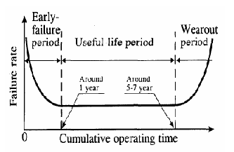 |
One aspect of disk failures that single-value metrics such as MTTF and AFR cannot capture is that in
real life failure rates are not constant [5]. Failure rates of hardware
products typically follow a ``bathtub curve'' with high failure rates at the beginning (infant
mortality) and the end (wear-out) of the lifecycle. Figure 2 shows the failure rate
pattern that is expected for the life cycle of hard drives [4,5,33].
According to this model, the first year of operation is characterized by early failures (or infant mortality).
In years 2-5, the failure rates are approximately in steady state, and then, after years 5-7, wear-out starts to kick in.
The common concern, that MTTFs do not capture infant mortality, has lead the International Disk
drive Equipment and Materials Association (IDEMA) to propose a new standard for specifying
disk drive reliability, based on the failure model depicted in Figure 2 [5,33].
The new standard requests that vendors provide four different MTTF estimates,
one for the first 1-3 months of operation, one for months 4-6, one for months 7-12, and
one for months 13-60.
The goal of this section is to study, based on our field replacement data, how disk replacement rates in
large-scale installations vary over a system's life cycle.
Note that we only see customer visible replacement. Any infant mortality failure caught in the
manufacturing, system integration or installation testing are probably not recorded in production
replacement logs.
The best data sets to study replacement rates across the system life cycle are HPC1 and the
first type of drives of HPC4.
The reason is that these data sets span a long enough time period (5 and 3 years, respectively) and
each cover a reasonably homogeneous hard drive population, allowing us to focus on the effect of age.
Figure 3:
ARR for the first five years of system HPC1's lifetime,
for the compute nodes (left) and the file system nodes (middle). ARR for the first type of drives in HPC4 as a function
of drive age in years (right).
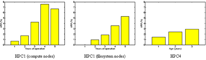 |
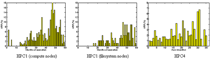
Figure 4:
ARR per month over the first five years of system HPC1's lifetime,
for the compute nodes (left) and the file system nodes (middle). ARR for the first type of drives in HPC4 as a function
of drive age in months (right).
 |
We study the change in replacement rates as a function of age at two different time granularities,
on a per-month and a per-year basis, to make it easier to detect both short term and
long term trends. Figure 3 shows the annual replacement rates for the disks
in the compute nodes of system HPC1 (left), the file system nodes of system HPC1 (middle)
and the first type of HPC4 drives (right), at a yearly granularity.
We make two interesting observations.
First, replacement rates in all years, except for year 1, are
larger than the datasheet MTTF
would suggest.
For example, in HPC1's second year, replacement rates are 20% larger than expected for the file system nodes,
and a factor of two larger than expected for the compute nodes. In
year 4 and year 5 (which are still within the nominal lifetime of these disks), the actual replacement
rates are 7-10 times higher than the failure rates we expected based on datasheet MTTF.
The second observation is that replacement rates are rising significantly over the years, even during
early years in the lifecycle. Replacement rates in HPC1 nearly double from year 1 to 2, or from
year 2 to 3.
This observation suggests that wear-out may start much earlier than expected, leading
to steadily increasing replacement rates during most of a system's useful life.
This is an interesting observation because it does not agree with the common assumption that
after the first year of operation, failure rates reach a steady
state for a few years, forming the ``bottom of the bathtub''.
Next, we move to the per-month view of replacement rates, shown in
Figure 4.
We observe that for the HPC1 file system nodes there are no replacements
during the first 12 months of operation, i.e. there's is no detectable infant mortality.
For HPC4, the ARR of drives is not higher in the first
few months of the first year than the last few months of the first year.
In the case of the HPC1 compute nodes, infant mortality is limited to the first month
of operation and is not above the steady state estimate of the datasheet MTTF.
Looking at the lifecycle after month 12, we again see continuously rising replacement rates,
instead of the expected ``bottom of the bathtub''.
Below we summarize the key observations of this section.
Observation 5: Contrary to common and proposed models, hard drive replacement rates do not enter
steady state after the first year of operation. Instead replacement rates seem to steadily
increase over time.
Observation 6: Early onset of wear-out seems to have a much stronger
impact on lifecycle replacement rates than infant mortality, as experienced by end customers,
even when considering only the first three or five years
of a system's lifetime. We therefore recommend that wear-out be incorporated into
new standards for disk drive reliability.
The new standard suggested by IDEMA does not take wear-out into account [5,33].
5 Statistical properties of disk failures
In the previous sections, we have focused on aggregate statistics, e.g. the average
number of disk replacements in a time period.
Often one wants more information on the statistical properties of the time between failures than just the mean.
For example, determining the expected time to failure for a RAID system requires an estimate on
the probability of experiencing a second disk failure in a short period, that is while
reconstructing lost data from redundant data.
This probability depends on the underlying probability distribution
and maybe poorly estimated by scaling an annual failure rate down to a few hours.
The most common assumption about the statistical characteristics of
disk failures is that they form a Poisson process, which implies
two key properties:
- Failures are independent.
- The time between failures follows an exponential distribution.
The goal of this section is to evaluate how realistic the above assumptions are.
We begin by providing statistical evidence that disk failures in
the real world are unlikely to follow a Poisson process.
We then examine each of
the two key properties (independent failures and exponential time
between failures) independently and characterize in detail how and where the Poisson assumption breaks.
In our study, we focus on the HPC1 data set, since this is the only data set that contains
precise timestamps for when a problem was detected (rather than just timestamps for when repair took place).
5.1 The Poisson assumption
Figure 5:
CDF of number of disk replacements per month in HPC1 computed across the entire lifetime of HPC1 (left) and computed for only years 2-3 (right)
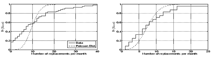 |
The Poisson assumption implies that the number of failures during a given
time interval (e.g. a week or a month) is distributed according to the
Poisson distribution. Figure 5 (left) shows the empirical CDF of the
number of disk replacements observed per month in the HPC1 data set, together with
the Poisson distribution fit to the data's observed mean.
We find that the Poisson distribution does not provide a good visual fit for the number of
disk replacements per month in the data, in particular for very small
and very large numbers of replacements in a month.
For example, under the Poisson distribution the probability of seeing
 failures in a given month is less than
0.0024, yet we see 20 or more disk replacements in nearly 20% of all months
in HPC1's lifetime.
Similarly, the probability of seeing zero or one failure in a given month is
only 0.0003 under the Poisson distribution, yet in 20% of all
months in HPC1's lifetime we observe zero or one disk replacement. failures in a given month is less than
0.0024, yet we see 20 or more disk replacements in nearly 20% of all months
in HPC1's lifetime.
Similarly, the probability of seeing zero or one failure in a given month is
only 0.0003 under the Poisson distribution, yet in 20% of all
months in HPC1's lifetime we observe zero or one disk replacement.
A chi-square test reveals that we can reject the hypothesis that
the number of disk replacements per month follows a Poisson distribution at the 0.05
significance level. All above results are similar when looking at the distribution
of number of disk replacements per day or per week, rather than per month.
One reason for the poor fit of the Poisson distribution might be that
failure rates are not steady over the lifetime of HPC1. We therefore repeat
the same process for only part of HPC1's lifetime. Figure 5 (right)
shows the distribution of disk replacements per month, using only data from
years 2 and 3 of HPC1. The Poisson distribution achieves a better fit
for this time period and the chi-square test cannot reject the Poisson
hypothesis at a significance level of 0.05.
Note, however, that this does not necessarily mean that the failure process
during years 2 and 3 does follow a Poisson process, since this would also require
the two key properties of a Poisson process (independent failures and
exponential time between failures) to hold.
We study these two properties in detail in the next two sections.
5.2 Correlations
In this section, we focus on the first key property of a Poisson process, the independence of
failures.
Intuitively, it is clear that in practice failures of disks in the same system are never completely independent.
The failure probability of disks depends for example on many factors, such as environmental factors, like temperature,
that are shared by all disks in the system. When the temperature in a machine room is far outside nominal
values, all disks in the room
experience a higher than normal probability of failure. The goal of this section is
to statistically quantify and characterize the correlation between disk replacements.
We start with a simple test in which we determine the correlation of the number of disk replacements
observed in successive weeks or months by computing the correlation coefficient between the number of replacements
in a given week or month and the previous week or month. For data coming from a Poisson processes
we would expect correlation coefficients to be close to 0. Instead we find significant levels of correlations,
both at the monthly and the weekly level.
The correlation coefficient between consecutive weeks
is 0.72, and the correlation coefficient between consecutive months is 0.79.
Repeating the same test using only the data of one year at a time, we still find significant
levels of correlation with correlation coefficients of 0.4-0.8.
Statistically, the above correlation coefficients indicate a strong correlation, but it
would be nice to have a more intuitive interpretation of this result.
One way of thinking of the correlation of failures is that
the failure rate in one time interval is predictive of the failure rate in the following time interval.
To test the strength of this prediction,
we assign each week in HPC1's life to one of three buckets, depending on the number
of disk replacements observed during that week, creating a bucket for weeks with small, medium, and large
number of replacements, respectively 1.
The expectation is that a week that follows a week with a ``small'' number of disk replacements is more
likely to see a small number of replacements, than a week that follows a week with a ``large''
number of replacements. However, if failures are independent, the number of replacements in a week will
not depend on the number in a prior week.
Figure 7:
Expected number of disk replacements in a week depending on the number of
disk replacements in the previous week computed across the entire lifetime of HPC1 (left) and computed for only year 3 (right).
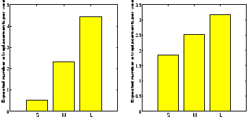 |
Figure 7 (left) shows the expected number of disk replacements in a week of HPC1's lifetime
as a function of which bucket the preceding week falls in.
We observe that the expected number of disk replacements in a week
varies by a factor of 9, depending on whether the preceding week falls into the first or third bucket,
while we would expect no variation if failures were independent.
When repeating the same process on the data of only year 3 of HPC1's lifetime,
we see a difference of a close to factor of 2 between the first and third bucket.
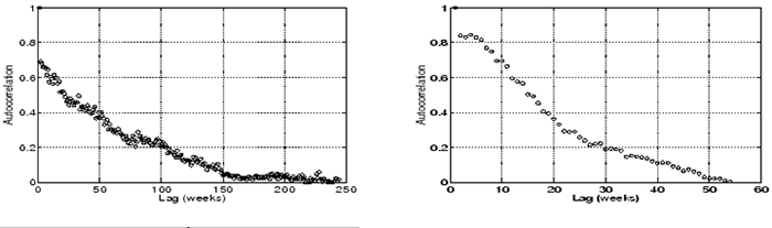
Figure 6:
Autocorrelation function for the number of disk replacements per week computed
across the entire lifetime of the HPC1 system (left) and computed across only one year of
HPC1's operation (right).
 |
So far, we have only considered correlations between successive time intervals, e.g. between
two successive weeks. A more general way to characterize correlations is to study
correlations at different time lags
by using the autocorrelation function. Figure 6 (left) shows the autocorrelation
function for the number of disk replacements per week computed across the HPC1 data set.
For a stationary failure process (e.g. data coming from a Poisson process) the autocorrelation
would be close to zero at all lags.
Instead, we observe strong autocorrelation even for large lags in the range of 100 weeks (nearly 2 years).
We repeated the same autocorrelation test for only parts of HPC1's lifetime and find similar levels of
autocorrelation. Figure 6 (right), for example, shows the autocorrelation function computed
only on the data of the third year of HPC1's life. Correlation is significant for lags in the range
of up to 30 weeks.
Another measure for dependency is long range dependence, as quantified by the Hurst exponent  .
The Hurst exponent measures how fast the autocorrelation functions drops with increasing lags.
A Hurst parameter between 0.5-1 signifies a statistical process with a long memory and a
slow drop of the autocorrelation function.
Applying several different estimators (see Section 2)
to the HPC1 data, we determine a Hurst exponent between 0.6-0.8 at the weekly granularity.
These values are comparable to Hurst exponents reported for Ethernet traffic, which is known to
exhibit strong long range dependence [16]. .
The Hurst exponent measures how fast the autocorrelation functions drops with increasing lags.
A Hurst parameter between 0.5-1 signifies a statistical process with a long memory and a
slow drop of the autocorrelation function.
Applying several different estimators (see Section 2)
to the HPC1 data, we determine a Hurst exponent between 0.6-0.8 at the weekly granularity.
These values are comparable to Hurst exponents reported for Ethernet traffic, which is known to
exhibit strong long range dependence [16].
Observation 7: Disk replacement counts exhibit significant levels of autocorrelation.
Observation 8: Disk replacement counts exhibit long-range dependence.
5.3 Distribution of time between failure
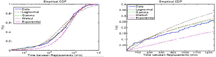
Figure 8:
Distribution of time between disk replacements across all nodes in HPC1.
 |
In this section, we focus on the second key property of a Poisson failure process, the exponentially distributed
time between failures.
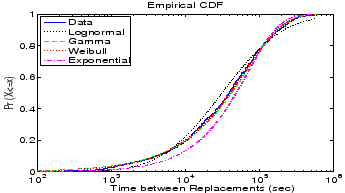
Figure 8 shows the empirical cumulative distribution
function of time between disk replacements as observed in the HPC1 system and
four distributions matched to it.
We find that visually the gamma and Weibull distributions are the best fit to the
data, while exponential and lognormal distributions provide a poorer fit.
This agrees with results we obtain from the negative log-likelihood, that indicate that
the Weibull distribution is the best fit, closely followed by the
gamma distribution.
Performing a Chi-Square-Test, we can reject the hypothesis that the underlying distribution is
exponential or lognormal at a significance level of 0.05.
On the other hand the hypothesis that the underlying distribution is a Weibull or a gamma cannot be
rejected at a significance level of 0.05.
Figure 8 (right) shows a close up of the empirical CDF and the distributions matched to it, for
small time-between-replacement values (less than 24 hours). The reason that this area is particularly interesting
is that a key application of the exponential assumption is in estimating the time until data loss in a RAID
system. This time depends on the probability of a second disk failure during reconstruction, a process
which typically lasts on the order of a few hours. The graph shows that the exponential distribution greatly
underestimates the probability of a second failure during this time period. For example, the probability of
seeing two drives in the cluster fail within one hour is four times larger under the real data, compared to the exponential
distribution. The probability of seeing two drives in the cluster fail within
the same 10 hours is two times larger under the real data, compared to the exponential distribution.
Figure 9:
Distribution of time between disk replacements across all nodes in HPC1 for only year 3 of operation.
 |
The poor fit of the exponential distribution
might be due to the fact that failure rates change over the lifetime of the system,
creating variability in the observed times between disk replacements
that the exponential distribution cannot capture.
We therefore repeated the above analysis considering only segments of HPC1's lifetime.
Figure 9 shows as one example the results from analyzing the time between disk replacements
in year 3 of HPC1's operation. While visually the exponential distribution now seems a slightly
better fit, we can still reject the hypothesis of an underlying exponential distribution at
a significance level of 0.05. The same holds for other 1-year and even 6-month segments of HPC1's lifetime.
This leads us to believe that even during shorter segments of HPC1's
lifetime the time between replacements is not realistically modeled by an exponential distribution.
While it might not come as a surprise that the simple exponential distribution does
not provide as good a fit as the more flexible two-parameter distributions,
an interesting question is what properties of the empirical time between failure
make it different from a theoretical exponential distribution.
We identify as a first differentiating feature that the data exhibits higher variability than a
theoretical exponential distribution. The data has a of 2.4, which is more than two times
higher than the of an exponential distribution, which is 1.
A second differentiating feature is that the time between disk replacements in the data
exhibits decreasing hazard rates.
Recall from Section 2.4 that the hazard rate function measures how the time since the last failure influences the expected time until the next failure.
An increasing hazard rate function predicts that if the time since a failure is long then the next failure
is coming soon. And a decreasing hazard rate function predicts the reverse.
The table below summarizes the parameters for the Weibull and gamma distribution that provided the best fit
to the data.
| |
Distribution / Parameters |
|
Weibull |
Gamma |
| |
Shape |
Scale |
Shape |
Scale |
| HPC1 compute nodes |
0.73 |
0.037 |
0.65 |
176.4 |
| HPC1 filesystem nodes |
0.76 |
0.013 |
0.64 |
482.6 |
| All HPC1 nodes |
0.71 |
0.049 |
0.59 |
160.9 |
Disk replacements in the filesystem nodes, as well as the compute nodes, and across all nodes, are fit best with
gamma and Weibull distributions with a shape parameter less than 1, a clear indicator of decreasing hazard rates.
Figure 10:
Illustration of decreasing hazard rates
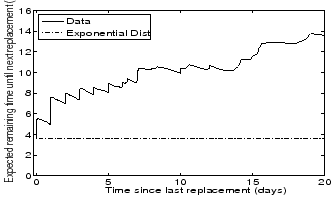 |
Figure 10 illustrates the decreasing hazard rates of the time between replacements
by plotting the expected remaining time
until the next disk replacement (Y-axis) as a function of the time since the last disk replacement (X-axis).
We observe that right after a disk was replaced the expected time until the next disk replacement becomes necessary
was around 4 days, both
for the empirical data and the exponential distribution.
In the case of the empirical data, after surviving for ten days without a disk replacement the expected
remaining time until the next replacement
had grown from initially 4 to 10 days; and after surviving for a total of 20 days without disk replacements the expected time until
the next failure had grown to 15 days. In comparison, under an exponential distribution the expected remaining
time stays constant (also known as the memoryless property).
Note, that the above result is not in contradiction with the increasing replacement rates we observed in
Section 4.2 as a function of drive age, since here we look at the distribution of the time
between disk replacements in a cluster, not disk lifetime distributions (i.e. how long did a drive live
until it was replaced).
Observation 9: The hypothesis that time between disk replacements follows
an exponential distribution can be rejected with high confidence.
Observation 10: The time between disk replacements has a higher variability
than that of an exponential distribution.
Observation 11: The distribution of time between disk replacements
exhibits decreasing hazard rates, that is, the expected remaining time until the next
disk was replaced grows with the time it has been since the last disk replacement.
6 Related work
There is very little work published on analyzing failures in real, large-scale storage systems,
probably as a result of the reluctance of the owners of such systems to release
failure data.
Among the few existing studies is the work by Talagala et al. [29],
which provides a study of error logs in a research prototype storage system used
for a web server and includes
a comparison of failure rates of different hardware components. They identify
SCSI disk enclosures as the least reliable components and SCSI disks as one
of the most reliable component, which differs from our results.
In a recently initiated effort, Schwarz et al. [28] have
started to gather failure data at the Internet Archive, which they plan to use to study
disk failure rates and bit rot rates and how they are affected by different environmental
parameters. In their preliminary results, they report ARR values of 2-6% and note
that the Internet Archive does not seem to see significant infant mortality. Both observations are
in agreement with our findings.
Gray [31] reports the frequency of uncorrectable read errors in disks
and finds that their numbers are smaller than vendor data sheets suggest.
Gray also provides ARR estimates for SCSI and ATA disks, in the range of
3-6%, which is in the range of ARRs that we observe for SCSI drives in our data sets.
Pinheiro et al. analyze disk replacement data from a large population
of serial and parallel ATA drives [23]. They report ARR values ranging from 1.7% to 8.6%,
which agrees with our results. The focus of their study is on the correlation between
various system parameters and drive failures. They find that while
temperature and utilization exhibit much less correlation with failures than expected,
the value of several SMART counters correlate highly with failures.
For example, they report that after a scrub error drives are 39 times more likely to fail
within 60 days than drives without scrub errors and that
44% of all failed drives had increased SMART counts in at least one of four specific counters.
Many have criticized the accuracy of MTTF based failure rate predictions and have pointed out
the need for more realistic models. A particular concern is the fact that
a single MTTF value cannot capture life cycle patterns [4,5,33].
Our analysis of life cycle patterns shows that this concern is justified, since
we find failure rates to vary quite significantly over even the first two to three years
of the life cycle.
However, the most common life cycle concern in published research is underrepresenting infant mortality.
Our analysis does not support this. Instead we observe
significant underrepresentation of the early onset of wear-out.
Early work on RAID systems [8] provided some statistical analysis
of time between disk failures for disks used in the 1980s, but didn't find sufficient evidence to reject the
hypothesis of exponential times between failure with high confidence.
However, time between failure has been analyzed for other, non-storage data in
several studies [11,17,26,27,30,32].
Four of the studies use distribution fitting and find the Weibull distribution
to be a good fit [11,17,27,32], which agrees with our results.
All studies looked at the hazard rate function, but come to
different conclusions. Four of them [11,17,27,32]
find decreasing hazard rates (Weibull shape parameter  ).
Others find that hazard rates are flat [30], or increasing [26].
We find decreasing hazard rates with Weibull shape parameter of 0.7-0.8. ).
Others find that hazard rates are flat [30], or increasing [26].
We find decreasing hazard rates with Weibull shape parameter of 0.7-0.8.
Large-scale failure studies are scarce, even when considering IT systems in general and not just storage systems.
Most existing studies are limited to only a few months of data,
covering typically only a few hundred failures [13,20,21,26,30,32].
Many of the most commonly cited studies on failure analysis stem from the
late 80's and early 90's, when computer systems where significantly
different from today [9,10,12,17,18,19,30].
7 Conclusion
Many have pointed out the need for a better understanding of what disk
failures look like in the field. Yet hardly any published work exists that
provides a large-scale study of disk failures in production systems.
As a first step towards closing this gap,
we have analyzed disk replacement data from a number of
large production systems, spanning more than 100,000 drives from
at least four different vendors, including drives with SCSI, FC and
SATA interfaces.
Below is a summary of a few of our results.
- Large-scale installation field usage appears to differ widely from nominal datasheet MTTF conditions.
The field replacement rates of systems were significantly larger than we expected based on datasheet MTTFs.
- For drives less than five years old, field replacement rates were larger
than what the datasheet MTTF suggested by a factor of 2-10.
For five to eight year old drives, field replacement rates were a factor of 30 higher than what the datasheet
MTTF suggested.
- Changes in disk replacement rates during the first five years of the lifecycle were more dramatic
than often assumed. While replacement rates are often expected to be in steady state in year
2-5 of operation (bottom of the ``bathtub curve''), we observed a continuous increase in replacement
rates, starting as early as in the second year of operation.
- In our data sets, the replacement rates of SATA disks are not worse than the
replacement rates of SCSI or FC disks. This may indicate that
disk-independent factors, such as operating conditions, usage and
environmental factors, affect replacement rates more than component specific
factors. However, the only evidence we have of a bad batch of disks was
found in a collection of SATA disks experiencing high media error rates. We
have too little data on bad batches to estimate the relative frequency of
bad batches by type of disk, although there is plenty of anecdotal evidence
that bad batches are not unique to SATA disks.
- The common concern that MTTFs underrepresent infant mortality
has led to the proposal of new standards that incorporate infant mortality [33].
Our findings suggest that the underrepresentation of the early onset of wear-out
is a much more serious factor than underrepresentation of infant mortality
and recommend to include this in new standards.
- While many have suspected that the commonly made assumption of exponentially
distributed time between failures/replacements is not realistic, previous studies have not found
enough evidence to prove this assumption wrong with significant statistical
confidence [8]. Based on our data analysis, we are able to reject the
hypothesis of exponentially distributed time between disk replacements with high confidence.
We suggest that researchers and designers use field replacement data, when possible, or
two parameter distributions, such as the Weibull distribution.
- We identify as the key features that distinguish the empirical distribution of time between disk replacements
from the exponential distribution, higher levels of variability and decreasing hazard rates.
We find that the empirical distributions are fit well by a Weibull distribution with
a shape parameter between 0.7 and 0.8.
- We also present strong evidence for the existence of correlations between disk replacement
interarrivals.
In particular, the empirical
data exhibits significant levels of autocorrelation and long-range dependence.
We would like to thank Jamez Nunez and Gary Grider from the High Performance Computing
Division at Los Alamos National Lab and Katie Vargo, J. Ray Scott and Robin Flaus from
the Pittsburgh Supercomputing Center for collecting and providing us with data and
helping us to interpret the data.
We also thank the other people and organizations, who have provided us with data, but would
like to remain unnamed. For discussions relating to the use of high end systems, we
would like to thank Mark Seager and Dave Fox of the Lawrence Livermore National Lab.
Thanks go also to the anonymous reviewers and our shepherd, Mary Baker,
for the many useful comments that helped improve the paper.
We thank the members and companies of the PDL Consortium (including APC,
Cisco, EMC, Hewlett-Packard, Hitachi, IBM, Intel, Network Appliance,
Oracle, Panasas, Seagate, and Symantec) for their interest
and support.
This material is based upon work supported by the Department of Energy under
Award Number DE-FC02-06ER257672and on research sponsored in part by the Army Research
Office, under agreement number DAAD19-02-1-0389.
Footnotes
- ... respectively 1
- More precisely, we choose the cutoffs between
the buckets such that each bucket contains the
same number of samples (i.e. weeks) by using the 33th percentile and the 66th percentile
of the empirical distribution as cutoffs between the buckets.
- ... DE-FC02-06ER257672
-
This report was prepared as an account of work sponsored by an agency of the United
States Government. Neither the United States Government nor any agency thereof, nor any of their
employees, makes any warranty, express or implied, or assumes any legal liability or responsibility
for the accuracy, completeness, or usefulness of any information, apparatus, product, or process
disclosed, or represents that its use would not infringe privately owned rights. Reference herein
to any specific commercial product, process, or service by trade name, trademark, manufacturer, or
otherwise does not necessarily constitute or imply its endorsement, recommendation, or favoring by
the United States Government or any agency thereof. The views and opinions of authors expressed
herein do not necessarily state or reflect those of the United States Government or any agency
thereof.
- 1
-
Personal communication with Dan Dummer, Andrei Khurshudov, Erik Riedel, Ron
Watts of Seagate, 2006.
- 2
-
G. Cole.
Estimating drive reliability in desktop computers and consumer
electronics systems. TP-338.1. Seagate.
2000.
- 3
-
Peter F. Corbett, Robert English, Atul Goel, Tomislav Grcanac, Steven Kleiman,
James Leong, and Sunitha Sankar.
Row-diagonal parity for double disk failure correction.
In Proc. of the FAST '04 Conference on File and Storage
Technologies, 2004.
- 4
-
J. G. Elerath.
AFR: problems of definition, calculation and measurement in a
commercial environment.
In Proc. of the Annual Reliability and Maintainability
Symposium, 2000.
- 5
-
J. G. Elerath.
Specifying reliability in the disk drive industry: No more MTBFs.
In Proc. of the Annual Reliability and Maintainability
Symposium, 2000.
- 6
-
J. G. Elerath and S. Shah.
Server class drives: How reliable are they?
In Proc. of the Annual Reliability and Maintainability
Symposium, 2004.
- 7
-
Sanjay Ghemawat, Howard Gobioff, and Shun-Tak Leung.
The Google file system.
In Proc. of the 19th ACM Symposium on Operating Systems
Principles (SOSP'03), 2003.
- 8
-
Garth A. Gibson.
Redundant disk arrays: Reliable, parallel secondary storage.
Dissertation. MIT Press.
1992.
- 9
-
J. Gray.
Why do computers stop and what can be done about it.
In Proc. of the 5th Symposium on Reliability in Distributed
Software and Database Systems, 1986.
- 10
-
J. Gray.
A census of tandem system availability between 1985 and 1990.
IEEE Transactions on Reliability, 39(4), 1990.
- 11
-
T. Heath, R. P. Martin, and T. D. Nguyen.
Improving cluster availability using workstation validation.
In Proc. of the 2002 ACM SIGMETRICS international conference on
Measurement and modeling of computer systems, 2002.
- 12
-
R. K. Iyer, D. J. Rossetti, and M. C. Hsueh.
Measurement and modeling of computer reliability as affected by
system activity.
ACM Trans. Comput. Syst., 4(3), 1986.
- 13
-
M. Kalyanakrishnam, Z. Kalbarczyk, and R. Iyer.
Failure data analysis of a LAN of Windows NT based computers.
In Proc. of the 18th IEEE Symposium on Reliable Distributed
Systems, 1999.
- 14
-
T. Karagiannis.
Selfis: A short tutorial.
Technical report, University of California, Riverside, 2002.
- 15
-
Thomas Karagiannis, Mart Molle, and Michalis Faloutsos.
Long-range dependence: Ten years of internet traffic modeling.
IEEE Internet Computing, 08(5), 2004.
- 16
-
Will E. Leland, Murad S. Taqqu, Walter Willinger, and Daniel V. Wilson.
On the self-similar nature of ethernet traffic.
IEEE/ACM Transactions on Networking, 2(1), 1994.
- 17
-
T.-T. Y. Lin and D. P. Siewiorek.
Error log analysis: Statistical modeling and heuristic trend
analysis.
IEEE Transactions on Reliability, 39(4), 1990.
- 18
-
J. Meyer and L. Wei.
Analysis of workload influence on dependability.
In Proc. International Symposium on Fault-Tolerant Computing,
1988.
- 19
-
B. Murphy and T. Gent.
Measuring system and software reliability using an automated data
collection process.
Quality and Reliability Engineering International, 11(5), 1995.
- 20
-
D. Nurmi, J. Brevik, and R. Wolski.
Modeling machine availability in enterprise and wide-area distributed
computing environments.
In Euro-Par'05, 2005.
- 21
-
D. L. Oppenheimer, A. Ganapathi, and D. A. Patterson.
Why do internet services fail, and what can be done about it?
In USENIX Symposium on Internet Technologies and Systems, 2003.
- 22
-
David Patterson, Garth Gibson, and Randy Katz.
A case for redundant arrays of inexpensive disks (RAID).
In Proc. of the ACM SIGMOD International Conference on
Management of Data, 1988.
- 23
-
E. Pinheiro, W. D. Weber, and L. A. Barroso.
Failure trends in a large disk drive population.
In Proc. of the FAST '07 Conference on File and Storage
Technologies, 2007.
- 24
-
Vijayan Prabhakaran, Lakshmi N. Bairavasundaram, Nitin Agrawal, Haryadi S.
Gunawi, Andrea C. Arpaci-Dusseau, and Remzi H. Arpaci-Dusseau.
Iron file systems.
In Proc. of the 20th ACM Symposium on Operating Systems
Principles (SOSP'05), 2005.
- 25
-
Sheldon M. Ross.
In Introduction to probability models. 6th edition. Academic Press.
- 26
-
R. K. Sahoo, R. K., A. Sivasubramaniam, M. S. Squillante, and Y. Zhang.
Failure data analysis of a large-scale heterogeneous server
environment.
In Proc. of the 2004 International Conference on Dependable
Systems and Networks (DSN'04), 2004.
- 27
-
B. Schroeder and G. Gibson.
A large-scale study of failures in high-performance computing
systems.
In Proc. of the 2006 International Conference on Dependable
Systems and Networks (DSN'06), 2006.
- 28
-
T. Schwarz, M. Baker, S. Bassi, B. Baumgart, W. Flagg, C. van Ingen, K. Joste,
M. Manasse, and M. Shah.
Disk failure investigations at the internet archive.
In Work-in-Progess session, NASA/IEEE Conference on Mass Storage
Systems and Technologies (MSST2006), 2006.
- 29
-
Nisha Talagala and David Patterson.
An analysis of error behaviour in a large storage system.
In The IEEE Workshop on Fault Tolerance in Parallel and
Distributed Systems, 1999.
- 30
-
D. Tang, R. K. Iyer, and S. S. Subramani.
Failure analysis and modelling of a VAX cluster system.
In Proc. International Symposium on Fault-tolerant computing,
1990.
- 31
-
C. van Ingen and J. Gray.
Empirical measurements of disk failure rates and error rates.
In MSR-TR-2005-166, 2005.
- 32
-
J. Xu, Z. Kalbarczyk, and R. K. Iyer.
Networked Windows NT system field failure data analysis.
In Proc. of the 1999 Pacific Rim International Symposium on
Dependable Computing, 1999.
- 33
-
Jimmy Yang and Feng-Bin Sun.
A comprehensive review of hard-disk drive reliability.
In Proc. of the Annual Reliability and Maintainability
Symposium, 1999.
This document was generated using the
LaTeX2HTML translator Version 2002 (1.67)
Copyright © 1993, 1994, 1995, 1996,
Nikos Drakos,
Computer Based Learning Unit, University of Leeds.
Copyright © 1997, 1998, 1999,
Ross Moore,
Mathematics Department, Macquarie University, Sydney.
|