James Lee Hafner, Veera Deenadhayalan, and KK Rao
John A. Tomlin
![[*]](footnote.png)
IBM Almaden Research Center
Yahoo! Research
hafner@almaden.ibm.com, [veerad,kkrao]@us.ibm.com
tomlin@yahoo-inc.com
For the scattered erasures, typically due to hard errors on the disk (or combinations of hard errors and disk loss), our methodology provides for one of two outcomes for the data on each lost sector. Either the lost data is declared unrecoverable (in the information-theoretic sense) or it is declared recoverable and a formula is provided for the reconstruction that depends only on readable sectors. In short, the methodology is both complete and constructive.
XOR-based erasures codes for disk arrays model lost data most coarsely
as loss of entire disks but more precisely as loss of entire symbols
of the code. In practice, a symbol typically maps to a ``strip'',
that is, multiple sequential sectors with one bit of the symbol
corresponding to one or (typically) more sectors and with each
different symbol residing on a different disk (this is not always the
case, but it is a common practice). The collection of related strips
is called a ``stripe''. To deal with disk failures, each erasure code
comes complete with a specific reconstruction algorithm that is highly
dependent on the code construction. For example, the
![]() -fault-tolerant X-code [10] is constructed
geometrically, with parity values computed along diagonal paths
through the data sectors. When two disks fail, the reconstruction
follows these diagonal paths, starting at some initial point; that is,
the reconstruction is both geometrically and recursively defined.
The BCP [1] code is less geometrically designed, but
still has a recursive reconstruction algorithm. More examples are
mentioned in Section 2.
-fault-tolerant X-code [10] is constructed
geometrically, with parity values computed along diagonal paths
through the data sectors. When two disks fail, the reconstruction
follows these diagonal paths, starting at some initial point; that is,
the reconstruction is both geometrically and recursively defined.
The BCP [1] code is less geometrically designed, but
still has a recursive reconstruction algorithm. More examples are
mentioned in Section 2.
Erasures then are seen as correlated sector failures: all sectors in a
strip are ``lost'' when the disk fails. However, increasing disk
capacity together with a fairly stable bit-error rate implies that
there is a significant probability of multiple uncorrelated or
scattered sector errors within a given stripe, particularly in
conjunction with one or more disk failures. For example, two disk
losses plus a sector loss may occur often enough that even a two-disk
fault tolerant code may not provide sufficient reliability. If all
correlated and uncorrelated erasures occur within at most ![]() disks
where
disks
where ![]() is the (disk) fault tolerance of the code, then one method
is to simulate loss of all affected disks and rebuild according to the
code-specific reconstruction algorithm. However, this has two
drawbacks. First, it is clear that this can be highly inefficient
since it requires either reconstruction of ``known'' or readable data
or it requires checking at each step of the process to see if a
reconstruction is required. More importantly, however, this approach
does not solve the more general problem when more than
is the (disk) fault tolerance of the code, then one method
is to simulate loss of all affected disks and rebuild according to the
code-specific reconstruction algorithm. However, this has two
drawbacks. First, it is clear that this can be highly inefficient
since it requires either reconstruction of ``known'' or readable data
or it requires checking at each step of the process to see if a
reconstruction is required. More importantly, however, this approach
does not solve the more general problem when more than ![]() disks have been affected with sector losses. In such a case, it is
quite possible that some or all of the lost sectors can be
reconstructed, though this is not obvious a priori from the
erasure correcting power of the code. For example, the 2-fault
tolerant EVENODD code only claims to recover from two lost disks, so
any additional sector loss typically means all lost data is declared
unrecoverable. In fact, on average, anywhere from 40-60% of the lost
sectors may be recovered in this situation.
disks have been affected with sector losses. In such a case, it is
quite possible that some or all of the lost sectors can be
reconstructed, though this is not obvious a priori from the
erasure correcting power of the code. For example, the 2-fault
tolerant EVENODD code only claims to recover from two lost disks, so
any additional sector loss typically means all lost data is declared
unrecoverable. In fact, on average, anywhere from 40-60% of the lost
sectors may be recovered in this situation.
In addition, while each erasure code provides a means to reconstruct entire strips (e.g., during a rebuild operation), to our knowledge, the literature does not contain any methods that explicitly address the problem of reconstructing a partial strip of lost data; such a need may arise in a host read operation to a failed disk during an incomplete rebuild operation. Of course, the strip reconstruction method could be applied in this case, but it is likely that such reconstruction will recover additional unnecessary lost sectors; that is, do more work than is required to service the host read, thereby adversely affecting performance. (This extra work may be worth the performance penalty in that the additional recovered sectors can be cached or added to the rebuild log, but that may not always be a desirable option.)
In this paper, we address both these problems. Our methodology is universal in that it can be applied to any erasure code of any fault tolerance. It applies to any failure scenario from full disk to scattered sectors to combinations of the two. It is based solely on the generator matrix for the erasure code. Consequently, a general erasure code reconstruction module could implement this methodology and use the generator matrix as one of its inputs. To emphasize the point, we address the problem of arbitrary sector (bit) erasures for any code designed with a strip (symbol) erasure failure model.
For the first problem of scattered (correlated and/or uncorrelated) sector loss, our methodology provides a mathematical guarantee: for each lost sector, either that sector's data is declared as (information-theoretically) unrecoverable (that is, a ``data loss event'') or the sector's data is declared recoverable and a reconstruction formula is generated. The reconstruction formula is a linear equation (XOR equation in case of XOR-based codes) involving known or readable data and parity sectors. In this respect, our methodology is both complete, constructive and universally applicable. It provides the best guarantee to meet the following requirement:
User Contract: For any erasure scenario, the storage system shall recover any and all lost data sectors that the erasure code is information-theoretically capable of recovering.
It should be noted that for ![]() -fault tolerant codes (e.g., RAID1,
RAID4 or RAID5), the solution to both these problems is quite simple
and obvious. Similarly, for Reed-Solomon codes [9]
where the symbol is mapped to bytes or words (not sets of sectors),
the standard Reed-Solomon procedure addresses both problems directly
as well. The more interesting cases then are non-Reed-Solomon multiple
fault-tolerant codes. Such codes are typically XOR-based as those have
the most practical application. Careful and complex analysis of a
specific code may produce a solution to this problem (and to our
second problem). However, our solutions are universal. It is also
clear that our methods can be extended to more general codes (e.g.,
some of the non-XOR codes in [3]). Furthermore, this
methodology can be applied not just for RAID controllers but any
application of these types of erasure codes such as dRAID (distributed
Redundant Arrangement of Independent Devices) node-based systems.
-fault tolerant codes (e.g., RAID1,
RAID4 or RAID5), the solution to both these problems is quite simple
and obvious. Similarly, for Reed-Solomon codes [9]
where the symbol is mapped to bytes or words (not sets of sectors),
the standard Reed-Solomon procedure addresses both problems directly
as well. The more interesting cases then are non-Reed-Solomon multiple
fault-tolerant codes. Such codes are typically XOR-based as those have
the most practical application. Careful and complex analysis of a
specific code may produce a solution to this problem (and to our
second problem). However, our solutions are universal. It is also
clear that our methods can be extended to more general codes (e.g.,
some of the non-XOR codes in [3]). Furthermore, this
methodology can be applied not just for RAID controllers but any
application of these types of erasure codes such as dRAID (distributed
Redundant Arrangement of Independent Devices) node-based systems.
For the second problem of partial strip reconstruction, we propose a hybrid solution: combine the inherent recursive method of the erasure code for full rebuild with the methodology for recovering scattered sectors. We also propose an alternative that is in many cases equivalent to the code-specific method, better in some cases and universally applicable to any erasure code.
Our methodology is based on principles of matrix theory and pseudo-inverses. Many codes (see [8,9]) use full inverses to prove both that their codes have the declared fault tolerance and to provide reconstruction formulas. However, they apply it only to recover full code symbols, under maximal failures (where unique inverses exist) and not to the more general bit-within-a-symbol (a.k.a, sector within a strip) level that we address in this work.
The paper is organized as follows. We close the introduction with some definitions. The next section contains a few remarks on related work. Section 3 contains a brief review of the concepts from linear algebra that we need, particularly the notion of pseudo-inverse. In Section 4 we present a brief description of the generator matrix and parity check matrix for an erasure code. Section 5 explains how we simulate scattered sector loss and how we determine reconstructability in addressing our first problem. Section 6 contains algorithms for constructing pseudo-inverse matrices. We develop our methods in a detailed example in Section 7. Section 8 outlines the hybrid method for partial strip reconstruction (our second problem) and includes experimental results. We conclude with a brief summary.
The two main results of this paper are (a) the application of pseudo-inverses of matrices to the problem of reconstruction of uncorrelated lost sectors and (b) a hybrid reconstruction that combines code-specific recursive reconstruction methods with this matrix method to efficiently reconstruct partial strips. To our knowledge neither of these problems has been specifically addressed in the literature. As remarked before, the theory of matrix inverses is used in the proof that some codes meet their declared strip (i.e., symbol) fault tolerance. For example, the Reed-Solomon code [8,9] proves fault tolerance by solving a system of linear equations. In this case, the matrix inverse method is used to solve for complete symbols (full strips in our terminology) under maximum failures. In contrast, our method addresses individual bits in symbols (i.e., elements) for any distribution of erased bits (within or beyond symbol fault tolerance). The binary BR [3] codes have a recursive solution to two full strip losses; the authors provide a closed form solution to the recursion. For the EVENODD code [2], the authors give a recursion and point out that it could be solved explicitly. An explicit solution to the recursion is equivalent to our matrix solution in the special case of full strip losses (again, our method has no such correlation requirements). The BCP [1], ZZS [11], X-code [10], and RDP [4] codes all have recursive reconstruction algorithms. The latter two (as well as the EVENODD code) are ``geometric'' and easy to visualize; the former are more ``combinatorial'' and less intuitive. In either case, these codes with recursive reconstruction algorithms are well-suited to our hybrid methodology. In addition, a variant of our hybrid method applies to any erasure codes suitable for disk arrays, with or without a recursive reconstruction algorithm.
In this section we recall and elaborate on some basic notions from
the theory of linear algebra over a binary field (which is assumed for
all operations from now on without further comment - the theory
extends easily to non-binary fields as well). A set of binary vectors
is linearly independent if no subset sums modulo ![]() to the zero
vector. Let
to the zero
vector. Let ![]() be a rectangular matrix of size
be a rectangular matrix of size ![]() with
with
![]() . The ``row rank'' of
. The ``row rank'' of ![]() is the maximum number of linearly
independent row vectors. The matrix
is the maximum number of linearly
independent row vectors. The matrix ![]() has ``full row rank'' if the
row rank equals
has ``full row rank'' if the
row rank equals ![]() (the number of rows). A ``null space'' for
(the number of rows). A ``null space'' for ![]() is
the set of all vectors that are orthogonal (have zero
dot-product) with every row vector of
is
the set of all vectors that are orthogonal (have zero
dot-product) with every row vector of ![]() . This is a vector
space closed under vector addition modulo
. This is a vector
space closed under vector addition modulo ![]() . A ``null space basis''
is a maximal set of linearly independent vectors from the null space.
If the null space basis has
. A ``null space basis''
is a maximal set of linearly independent vectors from the null space.
If the null space basis has ![]() vectors, then the entire null space
has
vectors, then the entire null space
has ![]() total non-zero vectors.
total non-zero vectors.
We will write the null space vectors as column vectors, to make matrix multiplication simpler to write down, though this is not the standard convention.
Let ![]() be a basis for the null space of
be a basis for the null space of ![]() . More precisely,
. More precisely, ![]() is
a matrix whose columns form a basis for the null space. If
is
a matrix whose columns form a basis for the null space. If ![]() has
full row rank, then
has
full row rank, then ![]() has dimensions
has dimensions ![]() where
where ![]() .
.
Suppose ![]() is full row rank. A ``right pseudo-inverse'' is a matrix
is full row rank. A ``right pseudo-inverse'' is a matrix
![]() (of size
(of size ![]() ) so that
) so that
More generally, let ![]() have row rank
have row rank ![]() , then a ``partial right
pseudo-inverse'' (or partial pseudo-inverse) is a matrix
, then a ``partial right
pseudo-inverse'' (or partial pseudo-inverse) is a matrix ![]() so that
so that
Let ![]() be a
be a ![]() basis for the null space basis for
basis for the null space basis for ![]() (perhaps padded with all-zero columns), and
(perhaps padded with all-zero columns), and ![]() some specific
partial pseudo-inverse for
some specific
partial pseudo-inverse for ![]() . As
. As ![]() varies over all binary
varies over all binary
![]() matrices, we have
matrices, we have
For each column of ![]() with a zero on the diagonal, the
corresponding column of
with a zero on the diagonal, the
corresponding column of ![]() can be replaced with the all-zero column
without affecting the partial pseudo-inverse property and in fact such
an action clearly improves the weight of
can be replaced with the all-zero column
without affecting the partial pseudo-inverse property and in fact such
an action clearly improves the weight of ![]() . Consequently, we add
this property to the definition of a partial pseudo-inverse.
. Consequently, we add
this property to the definition of a partial pseudo-inverse.
Strictly speaking, the term ``pseudo-inverse'' applies only to real or complex matrices and implies uniqueness (optimality in a metric sense). We overload the term here with a slightly different meaning - we allow for non-uniqueness and do not require optimality (most sparse).
In the next section we apply these notions to the problem of reconstruction of scattered sectors in a stripe.
In this section we recall the erasure code notions of ``generator matrix'' and ``parity check matrix''. These are the basic structures upon which we develop our methodology. For a basic reference, see [7].
The generator matrix ![]() of an erasure code converts the input
``word'' (incoming data) into a ``code word'' (data and parity). The
parity check matrix verifies that the ``code word'' contains
consistent data and parity (parity scrub). In the context of erasure
codes for disk arrays, the generator matrix actually provides much
more.
of an erasure code converts the input
``word'' (incoming data) into a ``code word'' (data and parity). The
parity check matrix verifies that the ``code word'' contains
consistent data and parity (parity scrub). In the context of erasure
codes for disk arrays, the generator matrix actually provides much
more.
The generator matrix is given a column block structure: each block
corresponds to a strip and each column within a block corresponds to
an element within the strip. If the column contains only a single ![]() ,
then the element contains user data. We call such a column an
``identity column'' because it is a column of an identity matrix. If
the column contains multiple
,
then the element contains user data. We call such a column an
``identity column'' because it is a column of an identity matrix. If
the column contains multiple ![]() s, then it corresponds to an element
which is the XOR sum of some set of user data elements; that is, the
element is a parity element. In other words, the generator matrix
specifies the data and parity layout on the strips, the logical
ordering of the strips within the stripe,
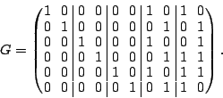
and the equations used to compute parity values. For
example, the generator matrix for the EVENODD(3,5) code with prime
s, then it corresponds to an element
which is the XOR sum of some set of user data elements; that is, the
element is a parity element. In other words, the generator matrix
specifies the data and parity layout on the strips, the logical
ordering of the strips within the stripe,
and the equations used to compute parity values. For
example, the generator matrix for the EVENODD(3,5) code with prime
![]() on
on ![]() disks is
disks is
Though it is not a requirement, the generator matrix for disk arrays typically has an identity column for each user data element (so that this data is always copied to the element's sectors verbatim in some strip and can then be read with minimal IO costs). In coding theory, a generator matrix of this form is called ``systematic''.
Let ![]() be a row vector of input user data values, then the row vector
be a row vector of input user data values, then the row vector
![]() , given by the expression
, given by the expression
If there are ![]() data elements input into the code and
data elements input into the code and ![]() parity
elements computed by the code, then the generator matrix has
dimensions
parity
elements computed by the code, then the generator matrix has
dimensions ![]() . (Note that
. (Note that ![]() is the total number of
data elements within a stripe, not the number of strips;
similarly,
is the total number of
data elements within a stripe, not the number of strips;
similarly, ![]() is the number of parity elements in the stripe, not the
number of parity strips.)
is the number of parity elements in the stripe, not the
number of parity strips.)
The ``parity check matrix'' ![]() has dimensions
has dimensions ![]() and can
be derived directly from the generator matrix (and vice-versa).
Communication channels use the parity check matrix to detect errors.
Each column corresponds to a parity element. After the data and
parity is read off the channel, the parity is XORed with the data as
indicated by its corresponding column to produce a ``syndrome''. If a
syndrome is not zero, an error has occurred (either in the received
parity symbol or in one of the dependent data symbols). For erasure
codes in disk arrays, this is a parity consistency check (or parity
scrub). In other words, with
and can
be derived directly from the generator matrix (and vice-versa).
Communication channels use the parity check matrix to detect errors.
Each column corresponds to a parity element. After the data and
parity is read off the channel, the parity is XORed with the data as
indicated by its corresponding column to produce a ``syndrome''. If a
syndrome is not zero, an error has occurred (either in the received
parity symbol or in one of the dependent data symbols). For erasure
codes in disk arrays, this is a parity consistency check (or parity
scrub). In other words, with ![]() as above, the test
as above, the test
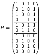
The parity check matrix is row blocked exactly corresponding to the
column blocks of ![]() (or
(or ![]() ) and it can be arranged to contain an
embedded identity matrix (corresponding to the parity elements) -
this is easy if
) and it can be arranged to contain an
embedded identity matrix (corresponding to the parity elements) -
this is easy if ![]() is systematic. The parity check matrix for the
example generator matrix
is systematic. The parity check matrix for the
example generator matrix ![]() above is
above is
In short, the generator matrix is used to compute the data and parity (and its layout) for storage on the disks. The parity check matrix can be used when all the data and parity are read off the disk (e.g., during parity scrub) to look for errors.
If a code can tolerate ![]() lost disks or strips, then
lost disks or strips, then ![]() must
have the property that if any
must
have the property that if any ![]() blocks of
blocks of ![]() are removed (or
zeroed), then the resulting matrix must have full row rank. The
parity check matrix is full column rank (because of the embedded
identity matrix).
are removed (or
zeroed), then the resulting matrix must have full row rank. The
parity check matrix is full column rank (because of the embedded
identity matrix).
Also, (3) implies that
In addition, it should be clear that if ![]() is systematic, then there
exists an
is systematic, then there
exists an ![]() matrix
matrix ![]() containing an embedded identity
matrix of size
containing an embedded identity
matrix of size ![]() so that
so that ![]() is a pseudo-inverse for
is a pseudo-inverse for ![]() .
.
![]() just picks off the embedded systematic portion of
just picks off the embedded systematic portion of ![]() . If
. If ![]() is not systematic, a pseudo-inverse
is not systematic, a pseudo-inverse ![]() can still be constructed,
but it will not be so simple (see Section 6.3).
can still be constructed,
but it will not be so simple (see Section 6.3).
In this section, we develop our theory for solving the first of our two problems: how to deal with uncorrelated sector loss. An example is given in Section 7
We indicated above that a ![]() -fault-tolerant code
-fault-tolerant code ![]() must have the
property that zeroing any
must have the
property that zeroing any ![]() blocks of
blocks of ![]() should leave
should leave ![]() full rank so that a complete pseudo-inverse for
full rank so that a complete pseudo-inverse for ![]() must exist. This
suggests that we can simulate correlated and/or uncorrelated
sector loss by zeroing or removing the associated individual
columns from
must exist. This
suggests that we can simulate correlated and/or uncorrelated
sector loss by zeroing or removing the associated individual
columns from ![]() . It should be clear that certain combinations of
uncorrelated sector losses will result in some or all data loss events
(some or all lost sectors having unrecoverable data); other
combinations may involve no data loss events. Our methodology will
determine, in a straightforward manner, exactly what sectors become
data loss events and for those that do not, will provide a
reconstruction formula for the data from these sectors.
. It should be clear that certain combinations of
uncorrelated sector losses will result in some or all data loss events
(some or all lost sectors having unrecoverable data); other
combinations may involve no data loss events. Our methodology will
determine, in a straightforward manner, exactly what sectors become
data loss events and for those that do not, will provide a
reconstruction formula for the data from these sectors.
Suppose we detect a set ![]() of failed sectors in a stripe
(correlated, perhaps because of disk failure, or uncorrelated, because
of medium errors, or a combination of these). Completely ignoring the
block structure of
of failed sectors in a stripe
(correlated, perhaps because of disk failure, or uncorrelated, because
of medium errors, or a combination of these). Completely ignoring the
block structure of ![]() , let
, let ![]() be a version of a generator matrix
be a version of a generator matrix
![]() , with zeroed columns corresponding to the sectors in
, with zeroed columns corresponding to the sectors in ![]() .
Suppose we can find a matrix
.
Suppose we can find a matrix ![]() of size
of size ![]() so that
so that
Proof.
Let ![]() be the vector
be the vector ![]() as in (2) but with zeros in
the positions corresponding to the lost elements (the zeroed columns
of
as in (2) but with zeros in
the positions corresponding to the lost elements (the zeroed columns
of ![]() ). Then it is clear that
). Then it is clear that
The fact that ![]() is uniquely determined by
is uniquely determined by ![]() means that any
zero diagonal entry of
means that any
zero diagonal entry of ![]() induces a zero in
induces a zero in ![]() ; this
corresponds to a data loss event. Any non-zero diagonal entry of
; this
corresponds to a data loss event. Any non-zero diagonal entry of
![]() induces a non-zero (not identically zero) data value in
induces a non-zero (not identically zero) data value in ![]() .
But the non-zero diagonal entries of
.
But the non-zero diagonal entries of ![]() corresponds to non-zero
columns of
corresponds to non-zero
columns of ![]() and the zero diagonal entries correspond to all-zero
columns of
and the zero diagonal entries correspond to all-zero
columns of ![]() . This proves part of the first and last statements.
. This proves part of the first and last statements.
Now consider a non-zero column of ![]() . Each non-zero bit in such a
column selects into an XOR formula a data or parity element from
. Each non-zero bit in such a
column selects into an XOR formula a data or parity element from
![]() . Because
. Because ![]() has zeros in row positions corresponding to
zeroed positions in
has zeros in row positions corresponding to
zeroed positions in ![]() , such a formula does not depend on any
lost data or parity element. The XOR formula then indicates that a
specific XOR sum of known data and parity elements equals the data
value associated to that column. That is, such a column provides a
formula for the reconstruction. This proves the rest of the first
statement in the theorem. The second claim of the theorem is clear.
, such a formula does not depend on any
lost data or parity element. The XOR formula then indicates that a
specific XOR sum of known data and parity elements equals the data
value associated to that column. That is, such a column provides a
formula for the reconstruction. This proves the rest of the first
statement in the theorem. The second claim of the theorem is clear.
![]()
We emphasize that this theorem makes no assumptions about the location of the failed sectors, whether they are correlated, uncorrelated or some of both. Consequently, the theorem can be applied to the case of full disk/strip losses (highly correlated) or even to the case where there is a lost sector on every strip (highly uncorrelated). It also does not depend on any special structure (for example geometric layout) of the erasure code. All the information we need is embedded within the generator matrix.
Recall that ![]() is not necessarily unique and that given a basis for
the null space of
is not necessarily unique and that given a basis for
the null space of ![]() , it is easy to construct, as
in (1), other pseudo-inverses that satisfy the same
properties as
, it is easy to construct, as
in (1), other pseudo-inverses that satisfy the same
properties as ![]() in the theorem. In the next section, we discuss
methods for constructing pseudo-inverses and bases for null spaces.
We use the null space bases for improving the sparseness of the
pseudo-inverse.
in the theorem. In the next section, we discuss
methods for constructing pseudo-inverses and bases for null spaces.
We use the null space bases for improving the sparseness of the
pseudo-inverse.
There are many possible algorithms for computing pseudo-inverses and null space bases. Fundamentally, they are equivalent though the data structures and approaches differ somewhat.
From now on, we use the label ![]() to indicate a matrix whose columns
form a null space basis for some zeroed matrix
to indicate a matrix whose columns
form a null space basis for some zeroed matrix ![]() , perhaps with
all-zero column vectors as padding. Furthermore, because we are
concerned only with uncorrelated sector loss, we ignore the block
structure of
, perhaps with
all-zero column vectors as padding. Furthermore, because we are
concerned only with uncorrelated sector loss, we ignore the block
structure of ![]() . As a result, we can assume without loss of
generality that the generator matrix
. As a result, we can assume without loss of
generality that the generator matrix ![]() has its systematic identity
submatrix in the first
has its systematic identity
submatrix in the first ![]() columns, with the parity columns in the
right most
columns, with the parity columns in the
right most ![]() columns - we call this ``left systematic''. (If not,
a permutation of the columns of
columns - we call this ``left systematic''. (If not,
a permutation of the columns of ![]() and corresponding column positions
in
and corresponding column positions
in ![]() ,
, ![]() , and
, and ![]() and row positions of
and row positions of ![]() ,
, ![]() and
and ![]() will reduce us to this case.)
will reduce us to this case.)
The input to our algorithms is the original generator matrix ![]() (and/or its parity check matrix
(and/or its parity check matrix ![]() ) and a list
) and a list ![]() of data or parity
elements which are declared lost (unreadable) in the stripe.
of data or parity
elements which are declared lost (unreadable) in the stripe.
The output of our algorithms will be two matrices ![]() and
and ![]() :
: ![]() is
a pseudo-inverse of
is
a pseudo-inverse of ![]() (obtained from
(obtained from ![]() by zeroing the columns
of
by zeroing the columns
of ![]() corresponding to the elements in
corresponding to the elements in ![]() ) and
) and ![]() is a basis for
the null space of
is a basis for
the null space of ![]() .
.
Our algorithms use ``column operations'' and/or ``row operations'' to manipulate matrices. Columns operations are equivalent to right multiplication by simple matrices (for rows, the operations are on the left). We consider three simplified column (or row) operations:
Our preferred algorithm, called the ``Column-Incremental''
construction, can be viewed as a dynamic or on-line algorithm. It
progressively updates data structures as new lost sectors are detected
(simulated by a incremental processing of the elements in ![]() ). In
Section 6.3, we outline some additional
constructions including static or off-line algorithms.
). In
Section 6.3, we outline some additional
constructions including static or off-line algorithms.
The algorithm presented here is an incremental algorithm. It starts
with a pseudo-inverse and null space basis for the matrix ![]() (in the
``good'' state) and incrementally removes (simulates) a lost data or
parity element, while maintaining the pseudo-inverse and null space
basis properties at each step. The algorithm is space efficient and
for most well-designed codes, has relatively few operations. It
requires space in
(in the
``good'' state) and incrementally removes (simulates) a lost data or
parity element, while maintaining the pseudo-inverse and null space
basis properties at each step. The algorithm is space efficient and
for most well-designed codes, has relatively few operations. It
requires space in ![]() only for the lost data elements (there is no
need to provide recovery formulas for parity elements as these can be
easily derived from the original formulas in the generator matrix -
alternatively, parity columns may be added to
only for the lost data elements (there is no
need to provide recovery formulas for parity elements as these can be
easily derived from the original formulas in the generator matrix -
alternatively, parity columns may be added to ![]() and so provide
additional formulas for a parity computation that reflect the lost
data elements). For clarity of exposition, our description is not
optimally space efficient; we leave that to the expert implementor.
and so provide
additional formulas for a parity computation that reflect the lost
data elements). For clarity of exposition, our description is not
optimally space efficient; we leave that to the expert implementor.
The process is reversible so long as the pseudo-inverse has full rank; that is, at any step, it is possible to model reconstruction of data values for lost elements (in any order) and compute a new pseudo-inverse and null space basis equivalent to one in which the recovered elements were never lost. This is described in Section 6.4
In this algorithm, column operations are performed on a workspace
matrix. The lost data or parity elements index a row of ![]() and
and ![]() .
.
Algorithm: Column-Incremental Construction
 .
.
A proof that this algorithm satisfies the required properties can be found in the appendix of the full technical report [5]. We make the following observations.
An alternative heuristic is the following: in the algorithm, a column
![]() of
of ![]() is chosen with a one in position
is chosen with a one in position ![]() among all such columns
of
among all such columns
of ![]() . This selected column is added to each of the others in
. This selected column is added to each of the others in ![]() .
This suggests that a heuristic for
.
This suggests that a heuristic for ![]() is to pick the one that
minimizes the total weight of the resulting columns. In
is to pick the one that
minimizes the total weight of the resulting columns. In
![]() -fault-tolerant codes, there are typically at most two such columns
to choose from, so this approach is equivalent to the one of minimal
weight above; this is not true for higher fault-tolerant codes.
-fault-tolerant codes, there are typically at most two such columns
to choose from, so this approach is equivalent to the one of minimal
weight above; this is not true for higher fault-tolerant codes.
This algorithm was a key ingredient to the results
of [6] where it was applied to measure performance
costs for a large variety of very different ![]() -fault-tolerant codes.
-fault-tolerant codes.
In this section we outline some approaches to implementing the optimizing step 3 in the Column-Incremental construction algorithm given above. As noted earlier, this step is not required to meet the User Contract stated in Section 1.
The following algorithm provides a systematic (though potentially very
expensive) approach to finding an optimal ![]() .
.
Algorithm: Improve ![]()
Of course, this is only practical if the null space has small enough
basis set. If the null space basis has very few vectors, then this
algorithm provides an exhaustive search solution to finding an optimal
![]() . In general, one can use any subset of the full null space to
find better, but perhaps not optimal, pseudo-inverses (in
Step 1 above, compute only some subset of the null
space). One simple choice, is to use only the basis vectors
themselves, or perhaps the basis vectors and all pairwise sums. It is
an open mathematical question if there are better algorithms for
finding the optimal
. In general, one can use any subset of the full null space to
find better, but perhaps not optimal, pseudo-inverses (in
Step 1 above, compute only some subset of the null
space). One simple choice, is to use only the basis vectors
themselves, or perhaps the basis vectors and all pairwise sums. It is
an open mathematical question if there are better algorithms for
finding the optimal ![]() than that given here. However, for the
extensive experiments we ran for [6], the difference
between optimal and near optimal was quite minimal.
than that given here. However, for the
extensive experiments we ran for [6], the difference
between optimal and near optimal was quite minimal.
There are alternative constructions that can be applied to computing
pseudo-inverses. Among them is a Row-Incremental variation that is
analogous to the Column-Incremental method described above but uses
row operations instead of column operations. Most of the steps are
the same as for the Column-Incremental construction. At
step 2b, for each one in positions ![]() in
the selected column
in
the selected column ![]() of
of ![]() , Sum and Replace row
, Sum and Replace row ![]() into row
into row ![]() of
of ![]() ; mirror this operation in
; mirror this operation in ![]() . At step 2c zero
row
. At step 2c zero
row ![]() in
in ![]() and
and ![]() and proceed to the next lost element. This
algorithm has all the same properties as the column variation
(including reversibility), but is typically more expensive, requiring
more row operations.
and proceed to the next lost element. This
algorithm has all the same properties as the column variation
(including reversibility), but is typically more expensive, requiring
more row operations.
Alternatively, there are both column and row versions that parallel
the classical algorithm for computing an inverse. Namely, start with
two matrices, the original generator matrix and an ![]() -identity
matrix. Zero the columns of the generator matrix and the identity
matrix corresponding to each lost data and parity element. Perform
column (or row) operations on the modified generator matrix to convert
it to column (or row) reduced echelon form. Parallel each of these
operations on the identity matrix; the resulting matrix contains both
the pseudo-inverse and null space basis. These variations are static,
off-line constructions as they utilize the complete set of lost
elements in the very first step. As before, the column version has
marginally less computation.
-identity
matrix. Zero the columns of the generator matrix and the identity
matrix corresponding to each lost data and parity element. Perform
column (or row) operations on the modified generator matrix to convert
it to column (or row) reduced echelon form. Parallel each of these
operations on the identity matrix; the resulting matrix contains both
the pseudo-inverse and null space basis. These variations are static,
off-line constructions as they utilize the complete set of lost
elements in the very first step. As before, the column version has
marginally less computation.
We do not give proofs for any of these constructions as they vary
only slightly from the proof of the Column-Incremental construction
found in the appendix of the full technical report [5].
The static algorithms can also
be used to construct an initial pseudo-inverse matrix for the full
generator matrix in the case when ![]() is not systematic.
is not systematic.
As mentioned, the incremental process can be used to start with a fully on-line stripe and, step by step, as medium errors are detected in the stripe, maintain a set of reconstruction formulas (or a declaration of non-reconstructability) for every data element in the stripe. As new medium errors are detected, the matrices are updated and new formulas are generated.
It might be useful to reverse the process. Suppose the array has had
some set of medium errors, but no data loss events and suppose a data
element is reconstructed by its formula in ![]() . If this reconstructed
data is replaced in the stripe, it would be helpful to update the
formulas to reflect this. There are two reasons for this. First, we
know we can replace the formula in
. If this reconstructed
data is replaced in the stripe, it would be helpful to update the
formulas to reflect this. There are two reasons for this. First, we
know we can replace the formula in ![]() by an identity column (we no
longer need the old formula). But second, it may be the case that
other lost elements can be reconstructed by better formulas that
contain this newly reconstructed element; we should update
by an identity column (we no
longer need the old formula). But second, it may be the case that
other lost elements can be reconstructed by better formulas that
contain this newly reconstructed element; we should update ![]() to
reflect this fact.
to
reflect this fact.
One approach would be to use any algorithm to recompute from scratch
the formulas for the revised set of sector losses. However, the
incremental algorithm suggests that we might be able to reverse the
process; that is, to update ![]() and
and ![]() directly to reflect the fact
that the data element has been reconstructed (e.g., its column in
directly to reflect the fact
that the data element has been reconstructed (e.g., its column in ![]() is replaced by an identity column).
is replaced by an identity column).
To fully reverse the incremental construction of the previous section, it must be the case that no information (in the information-theoretic sense) is lost through each step. Mathematically, this happens whenever we perform a non-invertible matrix operation, i.e., that corresponds to multiplication by a non-invertible matrix. This occurs essentially in only one place in the construction: whenever we can find no vector in the null space basis with a one in the desired row. This corresponds exactly to the case where we have data loss events.
Consequently, we have the following result: so long as we never
encounter the data loss branch, then (in principle), the sequence of
steps can be reversed. However, the algorithm we give below works
even after data loss events, so long as the restored element has a
reconstruction formula in ![]() , i.e., it is not itself a data
loss event . Note that it makes little sense to consider restoring
into the matrix an element corresponding to a data loss event (the
theorem says that this is theoretically impossible).
, i.e., it is not itself a data
loss event . Note that it makes little sense to consider restoring
into the matrix an element corresponding to a data loss event (the
theorem says that this is theoretically impossible).
The algorithm below performs this incremental restoration step in the case of a (recoverable) data element. Section 6.4.1 discusses the parity element case.
The input to this algorithm is a workspace matrix
![]() (possibly) generated by the incremental algorithm and
having the property that
(possibly) generated by the incremental algorithm and
having the property that
If the restored element is not from the set ![]() , then this algorithm
has no work to do, so we assume that the lost element is from
, then this algorithm
has no work to do, so we assume that the lost element is from ![]() .
.
Algorithm: Reverse Incremental Construction
This algorithm works because it takes the reconstruction formula for the data element and unfolds it back into the null space basis, then replaces the formula with an identity column.
The first optional step replaces any occurrence of the formula for
data element ![]() in the original
in the original ![]() by that element itself. In
particular, it explicitly restores into other columns a
dependence on the restored data element. In the process, it improves
the weight of these formulas.
by that element itself. In
particular, it explicitly restores into other columns a
dependence on the restored data element. In the process, it improves
the weight of these formulas.
This algorithm does not necessarily completely reverse the incremental algorithm in that it does not necessarily produce identical matrices going backward as were seen going forward. However, the difference will always be something in the null space.
A proof of this construction is given in the appendix of the full technical report [5].
To add a parity element back in to the matrices, we need to have the
original parity column from the generator matrix ![]() (for the data
columns, we know a priori that this column is an identity
column so we do not need to keep track of this externally). Suppose
that this parity is indexed by column
(for the data
columns, we know a priori that this column is an identity
column so we do not need to keep track of this externally). Suppose
that this parity is indexed by column ![]() in
in ![]() .
.
Take this parity column and for each ![]() in the column, sum together
(modulo 2) the corresponding columns of
in the column, sum together
(modulo 2) the corresponding columns of ![]() in
in ![]() and place the
result in an all-zero column of
and place the
result in an all-zero column of ![]() in
in ![]() . (This is exactly what we
did for a data column since there was only one such column!) Replace
the zero in position
. (This is exactly what we
did for a data column since there was only one such column!) Replace
the zero in position ![]() of this new column by
of this new column by ![]() . Replace column
. Replace column
![]() of
of ![]() by this parity column (restore it). (Again, this is
exactly what we did for a restored data column, except we also had to
set the
by this parity column (restore it). (Again, this is
exactly what we did for a restored data column, except we also had to
set the ![]() position in the inverse portion of
position in the inverse portion of ![]() to
to ![]() - in
the case of a parity column, no such position exists in the inverse
portion so this step is skipped.)
- in
the case of a parity column, no such position exists in the inverse
portion so this step is skipped.)
A proof is given in the appendix of the full technical report [5].
Consider the EVENODD(3,5) code [2] with prime ![]() ,
,
![]() total disks,
total disks, ![]() data disks and two parity disks. The data
and parity layout in the strips and stripe for one instance is given
in the following diagram:
data disks and two parity disks. The data
and parity layout in the strips and stripe for one instance is given
in the following diagram:
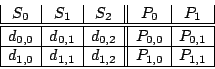
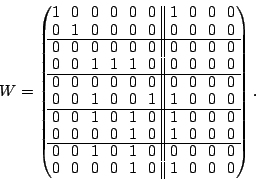
The generator matrix ![]() defined for this code is:
defined for this code is:
The parity check matrix ![]() is:
is:
For example, column ![]() of the parity check matrix says
of the parity check matrix says
More generally, we interpret these matrices in the following way. As
labeled above, we consider the user data values as a row vector
(ordered as already indicated):
The parity check matrix implies that
Any binary linear combination of the columns of ![]() will also be
orthogonal to all the vectors in
will also be
orthogonal to all the vectors in ![]() . E.g., take the binary sum (XOR)
of columns
. E.g., take the binary sum (XOR)
of columns ![]() and
and ![]() in
in ![]() :
:
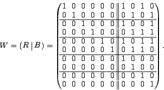
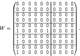
Suppose we loose strip ![]() and only data element
and only data element ![]() of
of ![]() in the EVENODD(3,5) code above. We then have a ``zeroed'' matrix
in the EVENODD(3,5) code above. We then have a ``zeroed'' matrix
![]() in the form:
in the form:

Using the data vector ![]() , we see that we have a revised set of
relationships:
, we see that we have a revised set of
relationships:
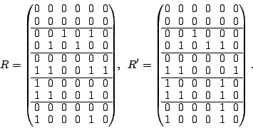
The following two matrices ![]() and
and ![]() are easily seen to be
pseudo-inverses for
are easily seen to be
pseudo-inverses for ![]() :
:
The columns of ![]() (or
(or ![]() ) correspond to the data elements as
ordered in the vector
) correspond to the data elements as
ordered in the vector ![]() . Each non-zero row corresponds to a
position in the vector
. Each non-zero row corresponds to a
position in the vector ![]() of known elements. Each all-zero row
matches a lost element in
of known elements. Each all-zero row
matches a lost element in ![]() . Each column represents an XOR
formula for reconstructing the data element to which it corresponds.
For example, to reconstruct
. Each column represents an XOR
formula for reconstructing the data element to which it corresponds.
For example, to reconstruct ![]() , we look at column
, we look at column ![]() of
of ![]() .
It indicates the following formula:
.
It indicates the following formula:
Because the code is MDS and can tolerate two disk/strip failures, it
is easy to see from dimension counting that ![]() has only one
non-zero vector in its null space. This vector turns out to be
has only one
non-zero vector in its null space. This vector turns out to be
The weight of each of the formulas for reconstructing data via ![]() is
at least as good as those in
is
at least as good as those in ![]() , consequently,
, consequently, ![]() is a better
solution than
is a better
solution than ![]() for our purposes. In fact, with only one vector in
the null space, it is clear that
for our purposes. In fact, with only one vector in
the null space, it is clear that ![]() is optimal.
is optimal.
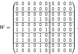
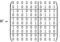
We start with the EVENODD(3,5) code as before and assume as above that
data elements ![]() ,
, ![]() , and
, and ![]() are lost from strips
are lost from strips
![]() and
and ![]() . These elements correspond to columns
. These elements correspond to columns ![]() of
of
![]() (and also to this set of rows in our workspace).
(and also to this set of rows in our workspace).
The initial workspace is

It can be checked that at each stage the claimed properties of
pseudo-inverse and null space of the intermediate results all hold.
It should be noted that this is not against the final ![]() but the intermediate
but the intermediate ![]() which we never write down).
which we never write down).
Now suppose in addition that element ![]() of strip
of strip ![]() is also
lost. This corresponds to a situation where sectors are lost from all
three data strips of the stripe. Nominally, the EVENODD(3,5) code can
only protect against losses on
is also
lost. This corresponds to a situation where sectors are lost from all
three data strips of the stripe. Nominally, the EVENODD(3,5) code can
only protect against losses on ![]() strips; we have three partial
strips, a case not covered in the literature.
strips; we have three partial
strips, a case not covered in the literature.
The element ![]() corresponds to
corresponds to ![]() . We select column
. We select column ![]() ,
perform the operations in the algorithm and the result is
,
perform the operations in the algorithm and the result is
Observe that any column corresponding to a data element that is not lost has remained unchanged as an identity column. In addition, even though we have lost sectors in three strips, all sectors are still recoverable.
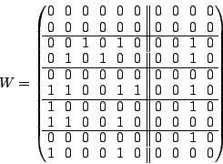
If we further assume that data element ![]() (corresponding to row
(corresponding to row ![]() ) is also lost, we can continue the
algorithm. In this case, there is no null space basis vector with a
one in this row. So, the algorithm says to zero all columns in
) is also lost, we can continue the
algorithm. In this case, there is no null space basis vector with a
one in this row. So, the algorithm says to zero all columns in ![]() with a one in this row (that is, columns
with a one in this row (that is, columns ![]() ). This produces
the matrix
). This produces
the matrix
We start with the result of our incremental construction example in
equation (8) where we have lost sectors ![]() ,
,
![]() ,
, ![]() and
and ![]() corresponding to columns
corresponding to columns
![]() of
of ![]() . Suppose we have reconstructed data element
. Suppose we have reconstructed data element
![]() of column
of column ![]() (which is not the last element we
simulated as lost). The reverse incremental algorithm above has the
following steps. (We include the optional steps for completeness.)
(which is not the last element we
simulated as lost). The reverse incremental algorithm above has the
following steps. (We include the optional steps for completeness.)
First, we examine each of the first six columns to see if column ![]() is contained in it. Column
is contained in it. Column ![]() has one's in positions
has one's in positions ![]() .
No other column has ones in all these positions, so we continue to
the next step.
.
No other column has ones in all these positions, so we continue to
the next step.
Next we select the all-zero column ![]() and set position
and set position ![]() in this
column and in column
in this
column and in column ![]() to the value
to the value ![]() , then we swap these two
columns:
, then we swap these two
columns:

Note that our final result does have an identity column in position
![]() so we have restored this data element.
so we have restored this data element.
In this section we introduce the hybrid reconstruction method. It applies the reconstruction methodology based on the matrix method in another way to address the problem of partial strip reconstruction.
Suppose the array's erasure code can tolerate two strip failures. Most such erasure codes have a recursive algorithm defined for reconstructing the two lost strips. This can be quite efficient for rebuild of both lost strips in their entirety. The steps are generally quite simple and explicitly assume use of intermediate reconstructed elements. However, such a method will be very code-dependent; that is, the recursion will depend on the specific code layout and parity formulas. On the other hand, the matrix methodology above is completely generic. If applied without the Reverse Incremental construction, no intermediate results are used; consequently, the amount of XOR computation could be quite large compared to a recursive method. But the Reverse Incremental construction would directly take advantage of intermediate results and improve overall XOR computation costs. In fact, if applied appropriately (as a special case of our algorithm below), the matrix method (including the Reverse Incremental construction) would reduce to the recursive method in most cases (and be very similar in all others).
Now consider a host request to read a single block from one of the two lost strips (prior to completion of any background process to reconstruct the stripe). If the element is very deep into the recursion, a number of intermediate reconstructions (of lost elements) must take place; these intermediate results are not needed for the immediate host request and, though they can be cached, are potentially extraneous work for the task at hand. The matrix method above, however, gives a (near) optimal formula for direct reconstruction of any single element without reconstruction of any additional elements.
We see that for single element reconstruction, the generic direct method of the matrix methodology is generally more efficient than the recursive method provided with a specific code. Conversely, for reconstruction of all lost elements the generally preferred method is the recursive method (either explicitly using the code's specific theory or implicitly using the matrix method together with the Reverse Incremental construction).
We now consider the problem of reconstructing a partial strip, say, to
satisfy a host read for multiple consecutive blocks that span multiple
elements in a strip. We assume that multiple strips are lost (though
that is not a requirement at all). The above discussion suggests that
neither the direct nor the recursive methods may be optimal to address
this problem efficiently. We propose the following algorithm. The
input to the algorithm is the set of lost sectors ![]() , the parity
check matrix (or the generator matrix) and a subset
, the parity
check matrix (or the generator matrix) and a subset ![]() of
of ![]() containing sectors to reconstruct (we assume that no element in
containing sectors to reconstruct (we assume that no element in ![]() is
a data loss event). The output is the data values for the elements in
is
a data loss event). The output is the data values for the elements in
![]() . That is,
. That is, ![]() is the complete set of lost sectors and
is the complete set of lost sectors and ![]() is that
partial set we need to reconstruct.
is that
partial set we need to reconstruct.
Algorithm: Code-specific Hybrid Reconstruction
Essentially, this algorithm uses the direct method to jump into the
recursion at the first point the recursion intersects the set ![]() (thereby avoiding reconstruction of unneeded values). The optional
step 2(d)i ensures that we have factored into the direct
reconstruction formulas all values reconstructed to this point,
thereby allowing these elements to be used in later reconstruction
formulas (lowering XOR computational costs).
(thereby avoiding reconstruction of unneeded values). The optional
step 2(d)i ensures that we have factored into the direct
reconstruction formulas all values reconstructed to this point,
thereby allowing these elements to be used in later reconstruction
formulas (lowering XOR computational costs).
During step 2c, we can avoid physical reconstruction
of intermediate steps in the recursion that are not in set ![]() (that is, not immediately required for the host) by logically
collapsing the recursion equations. That is, we combine the steps of
the recursions to get from
(that is, not immediately required for the host) by logically
collapsing the recursion equations. That is, we combine the steps of
the recursions to get from ![]() to
to ![]() . This has two advantages.
First, it avoids a computation and temporary memory store of any
unneeded intermediate result. Second, the combination can eliminate
the need for some data or parity values that appear multiply (an even
number of times) in the set of recursive formulas. This avoids a
possible disk read to access this data as well as the memory bandwidth
costs to send this data into and out of the XOR engine multiple times.
. This has two advantages.
First, it avoids a computation and temporary memory store of any
unneeded intermediate result. Second, the combination can eliminate
the need for some data or parity values that appear multiply (an even
number of times) in the set of recursive formulas. This avoids a
possible disk read to access this data as well as the memory bandwidth
costs to send this data into and out of the XOR engine multiple times.
Step 2b looks for efficient ways to utilize the
recursion. If none exist, we reapply the direct method (updated,
perhaps) to jump back into the recursion at some other point in ![]() of
minimal direct costs.
of
minimal direct costs.
Together, these steps enable efficient reconstruction of only those
elements that are needed (those in ![]() ) and no others. There are two
special cases: (a) if
) and no others. There are two
special cases: (a) if ![]() is a singleton, then this method will apply
the direct method in the first step then exit; (b) if
is a singleton, then this method will apply
the direct method in the first step then exit; (b) if ![]() is the union
of all the elements on all lost strips, then the algorithm will
default to the application of the recursion alone. We see then that
this algorithm interpolates between these two extremes to find
efficient reconstruction of partial strips. (Note that
is the union
of all the elements on all lost strips, then the algorithm will
default to the application of the recursion alone. We see then that
this algorithm interpolates between these two extremes to find
efficient reconstruction of partial strips. (Note that ![]() need not
be a partial strip, but that is the most likely application.)
need not
be a partial strip, but that is the most likely application.)
More generically, we can apply the following algorithm as a means to efficiently solve the same problem, without reference to the specific recursion of the code (assuming it has one).
Algorithm: Generic Hybrid Reconstruction
It is not hard to see that in the presense of a straight forward recursion, the code-specific and generic hybrid methods will produce similar results (perhaps in different order of reconstruction, but with the same or similar costs). The application of the recursion in step 2c in the code-specific algorithm implicitly applies the Reverse Incremental algorithm.
Figure 1 shows the advantages of this hybrid method
for the EVENODD code [2]. The chart shows the
XOR costs (total number of XOR input and output variables) for disk
array sizes from ![]() to
to ![]() . These numbers are the average over all
1/2-strip-sized (element-aligned) host read requests to lost strips
and averaged over all possible
. These numbers are the average over all
1/2-strip-sized (element-aligned) host read requests to lost strips
and averaged over all possible ![]() strip failures. They are
normalized to the Direct XOR costs. The figure shows that the direct
cost is generally (except for very small arrays) more expensive than
application of the recursive method (as one would expect for long
reads), but it also shows that the Hybrid method is significantly more
efficient than both.
strip failures. They are
normalized to the Direct XOR costs. The figure shows that the direct
cost is generally (except for very small arrays) more expensive than
application of the recursive method (as one would expect for long
reads), but it also shows that the Hybrid method is significantly more
efficient than both.
![\includegraphics[width=\graphicwidth,bb=57 401 504 717]{figs/hybrid_ks_rj}](img147.png)
|
We developed a language to model uncorrelated and/or correlated loss of sectors (or elements) in arbitrary array codes. We provided a direct methodology and constructive algorithms to implement a universal and complete solution to the recoverability and non-recoverability of these lost sectors. This method and algorithm meets the User Contract that says that what is theoretically recoverable shall be recovered. Our solution can be applied statically or incrementally. We demonstrated the power of the direct method by showing how it can recover data in lost sectors when these sectors touch more strips in the stripe than the fault tolerance of the erasure code. The direct method can be joined with any code-specific recursive algorithm to address the problem of efficient reconstruction of partial strip data. Alternatively, the incremental method can be reversed when some data is recovered to provide a completely generic method to address this same partial strip recovery problem. Finally, we provided numerical results that demonstrate significant performance gains for this hybrid of direct and recursive methods.
The authors thank Tapas Kanungo and John Fairhurst for their contributions to this work and the reviewers for helpful suggestions to improve the exposition.
This document was generated using the LaTeX2HTML translator Version 2002-2-1 (1.71)
Copyright © 1993, 1994, 1995, 1996,
Nikos Drakos,
Computer Based Learning Unit, University of Leeds.
Copyright © 1997, 1998, 1999,
Ross Moore,
Mathematics Department, Macquarie University, Sydney.
The command line arguments were:
latex2html -split 0 -show_section_numbers -local_icons matrix_hybrid_fast05
The translation was initiated by on 2005-10-07