Experimental Analysis Polus : Growing Storage Meta-level operations

Experimental Setup

In the experimental setup, a SAN file system simulator is being used as the managed system. For the management software, we use an implementation of the Polus toolkit and compare it with its rule-based ECA counterpart. The Polus toolkit is built using ABLE (Agent Building and Learning Environment) [4]. ABLE provides the basic building blocks for Polus, namely learning algorithms such as neural networks, self-organizing map, JDBC connectivity for interfacing with the database, and data filters. The Polus modules are implemented as Java beans or agents. The implementation consist of agents for: Specifications (input), Reasoning, Learning, Sensors and Actuators. The rest of the section describes the implementation of the file system simulator.

The entities within the SAN file-system simulator are similar to those introduced in Section 2. The cost of atomic operations used in the simulator are shown in table 1. The simulator models the following actions that are invoked by the management software via actuators: Pre-fetch size tuning, Data replication, Backup and Clean-delay interval. I/O operations within the SAN file system are invoked by the client and can have multiple possible paths, depending on whether the data is cache or not. The simulator considers the following paths:

MHDH: Metadata and data hit in the client

MHDM: Metadata hit and data miss in client

MMDM: Metadata and data miss in the client

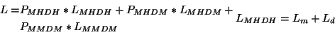
The summation of each of these probabilities of the invocation paths $P_{MHDH} + P_{MHDM} + P_{MMDM} = 1$

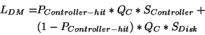
The average I/O latency is given by:

$$\begin{gather*}\begin{split}L = & P_{MHDH}*L_{MHDH}+P_{MHDM}*L_{MHDM}+ \\ & P_{MMDM}*L_{MMDM} \end{split}L_{MHDH}=L_{m} + L_{d}\end{gather*} L_{MHDM}=L_{m}+L_{DM} \begin{gather*}\begin{split}L_{DM}= & P_{Controller-hit}*Q_{C}*S_{Controller}+ \\ & (1-P_{Controller-hit})*Q_{C}*S_{Disk}\\ \end{split}\end{gather*} L_{MMDM}=Queue\_depth_{Server}*S_{Server} + L_{DM}$$

 

Table 1: Cost of atomic operations in the file system simulator

Operation	Cost
Size of metadata object	1000 bytes
Latency to access from metadata cache ($L_{m}$)	$20\ \mu sec$
Latency to read from datacache ($L_{d}$)	$20\ \mu sec$
Service time of server ( $S_{server}$)	$420\ \mu sec$
Service time from controller cache ( $S_{controller}$)	$0.6\ msec$
Service time of disk ($S_{disk}$)	$6\ msec$
Queue depth at controller ($Q_{C}$)	$256$(max)
Size of metadata cache	$128$MB
Size of data cache	1 GB
Size of controller cache	256 MB

 

 

Table 2: Modeling actions within the file system simulator

Action	Description	Invocation path parameters affected	Resources affected
Prefetching	Readahead of data and metadata	$P_{MHDH}$and $P_{MHDM}$	Data cache, metadata cache and interconnect bandwidth
Replication	Creates replica of data on a different volume in the controller	$Q_{C}$	Storage space (ignoring transient effects)
Data backup	Consider only transient effects since we are not considering availability	$P_{MHDH}$, $P_{MHDM}$, $P_{MMDM}$ $Q_{C}$, $Q_{Server}$	Memory, interconnect bandwidth and storage space
Clean delay	Frequency at which dirty buffers are flushed to disks	Only for writes - $P_{MHDH}$ bursty traffic for storage controller $Q_{C}$:	Metadata cache and data cache (metadata cannot be evicted till data is written)

 

The values for probabilities such as $P_{MHDH}$, and $P_{Controller-hit}$are modeled by representing the caches as finite sized-arrays and keeping track of data blocks in the elements. Similarly, the average queue depth such as $Q_{C}$are actually modeled by using service time to complete each request.

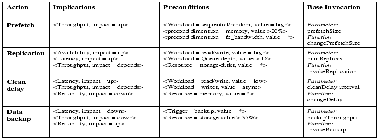
Each action is modeled to reflect its impact on the invocation path, system resources and changes in the workload characteristics (table 2). To activate the actions in the file system simulator, specifications are fed into Polus and rule-based management. The specifications for a rule-based system consist of ECAs that describe the system-behavior for different system-states. The ECA specifications in this example run into 7 pages (76 rules). The exact Polus specifications that are fed are given in figure 8.

Figure: Specifications fed to the Polus framework

Experimental Analysis Polus : Growing Storage Meta-level operations