
An EW-Array employs all three of the above techniques. A large ![]() value allows for more efficient writes. A large
value allows for more efficient writes. A large ![]() value more
aggressively reduces the seek cost. A large
value more
aggressively reduces the seek cost. A large ![]() value more
aggressively reduces the rotational cost of reads. Given a total
budget of
value more
aggressively reduces the rotational cost of reads. Given a total
budget of ![]() disks and the constraint
disks and the constraint
![]() , one must carefully balance these three
dimensions to optimize the overall performance.
The decision of how to configure these three dimensions is influenced
by both the workload and disk characteristics. A workload that has a
small read-to-write ratio and little idle time demands a large
dilution factor
, one must carefully balance these three
dimensions to optimize the overall performance.
The decision of how to configure these three dimensions is influenced
by both the workload and disk characteristics. A workload that has a
small read-to-write ratio and little idle time demands a large
dilution factor ![]() so that more resources are devoted to
speeding up writes. Disks with large seek delays
demand a large striping factor
so that more resources are devoted to
speeding up writes. Disks with large seek delays
demand a large striping factor ![]() , while disks with large
rotational delay demand a large mirroring factor
, while disks with large
rotational delay demand a large mirroring factor ![]() .
.
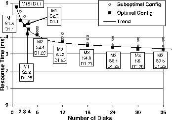
In this section, we explore the impact of array configurations using a simple synthetic workload (that is part of the Intel ``Iometer'' benchmark [15]). More complex workloads are explored in Section 6. In each of the test runs, the length of the queue of the outstanding requests is kept at a constant. This is accomplished by adding a new request to the queue as soon as an old one is retired from it. Different queue lengths emulate different degree of idleness in the system. In all runs, the read/write ratio is 50/50.
Figure 2 compares the latency of alternative
EW-Array configurations.
In these experiments, the number of outstanding requests is one so
there is no queueing.
As a result,
a relatively small dilution factor (![]() ) is generally
sufficient for absorbing
the writes while a relatively large
) is generally
sufficient for absorbing
the writes while a relatively large
![]() product improves
read latency. A properly configured 4-disk EW-Array halves the
latency achieved on a single-disk conventional system.
Note that many of the configurations in Figure 2
have fractional values for
product improves
read latency. A properly configured 4-disk EW-Array halves the
latency achieved on a single-disk conventional system.
Note that many of the configurations in Figure 2
have fractional values for ![]() and
and ![]() , yet
, yet
![]() is
always integral. That means each replica stripes data across
is
always integral. That means each replica stripes data across
![]() disks. On each of those disks, only
disks. On each of those disks, only ![]() fraction of the tracks are
actually used to store data, and utilization of those tracks is
fraction of the tracks are
actually used to store data, and utilization of those tracks is ![]() .
.
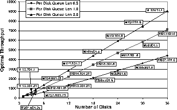
Figure 3 shows how the throughput of optimally
configured EW-Arrays scales with an increasing number of disks.
We vary the number of outstanding requests per disk to emulate different
load levels.
For a fixed number of disks,
as we raise the request arrival rate, a progressively larger dilution factor
![]() is needed to absorb the disk writes that can no longer be masked
by idle periods.
is needed to absorb the disk writes that can no longer be masked
by idle periods.
 |
 |