
A Case for Machine Learning to Optimize Multicore Performance
Archana Ganapathi, Kaushik Datta, Armando Fox and David Patterson
Computer Science Division, University of California at Berkeley
{archanag, kdatta, fox, pattrsn}@cs.berkeley.edu
Multicore architectures are becoming increasingly complex due to higher core counts, varying degrees of multithreading, and memory hierarchy complexity. This rapidly evolving landscape has made it difficult for compilers to keep pace. As a result, compilers are unable to fully utilize system resources and hand-tuning is neither scalable nor portable. Auto-tuning has emerged as a solution that can be applied across platforms for performance optimization. Auto-tuning first identifies a set of useful optimizations and acceptable parameter ranges using hardware expertise and application-domain knowledge. Then it searches the parameter space to find the best performing configuration. In the last decade, auto-tuning has been successfully used to tune scientific kernels for both serial [9,11] and multicore processors [12,8].
Auto-tuning is scalable, automatic, and can produce high-quality code that is several times faster than a naïve implementation [6]. Unfortunately it suffers from two major drawbacks. The first is the size of the parameter space to explore: state-of-the-art auto-tuners that consider only a single application, a single compiler, a specific set of compiler flags, and homogeneous cores may explore a search space of over 40 million configurations [8]. This search would take about 180 days to complete on a single machine. If the auto-tuner considers alternative compilers, multichip NUMA systems, or heterogeneous hardware, the search becomes prohibitively expensive. Even parallel exploration of multiple configurations (e.g. in a supercomputing environment) achieves only linear speedup in the search, so most auto-tuners prune the space by using heuristics of varying effectiveness.
The second drawback is that most auto-tuners are only trying to minimize overall running time. Given that power consumption is a proximate cause of the multicore revolution, and a vital metric for tuning embedded devices, it is important to tune for energy efficiency as well. A performance-optimal configuration is not necessarily energy-optimal and vice versa.
We propose to address both these drawbacks using statistical machine learning (SML). SML algorithms allow us to draw inferences from automatically constructed models of large quantities of data [10]. The advantage of SML-based methodologies is that they do not rely on application or micro-architecture domain knowledge. Additionally, several SML methodologies allow us to simultaneously tune for multiple metrics of success [3]. We are able to reduce the half-year long search to two hours while achieving performance at least within 1% of and up to 18% better than a that achieved by a human expert.
We are inspired by the success of the systems community in using SML techniques to detect and diagnose failures and to predict performance [15,14,3]. The systems community has had to overcome hurdles to applying SML [10] that may be absent in the multicore/architecture domain. In contrast to the difficulty of collecting systems data, the architecture community has the advantage that real data can be obtained quickly using commodity hardware. Furthermore, the architecture community has a long-established culture of designing for testability and measurability via programmer-visible performance counters, making it is easier to find "ground truth". Lastly, since the architecture community tends to optimize applications with exclusive access to hardware, the SML models need not adapt to varying machine usage patterns and externally-imposed load conditions. As a result of these advantages, we see a great opportunity for using SML.
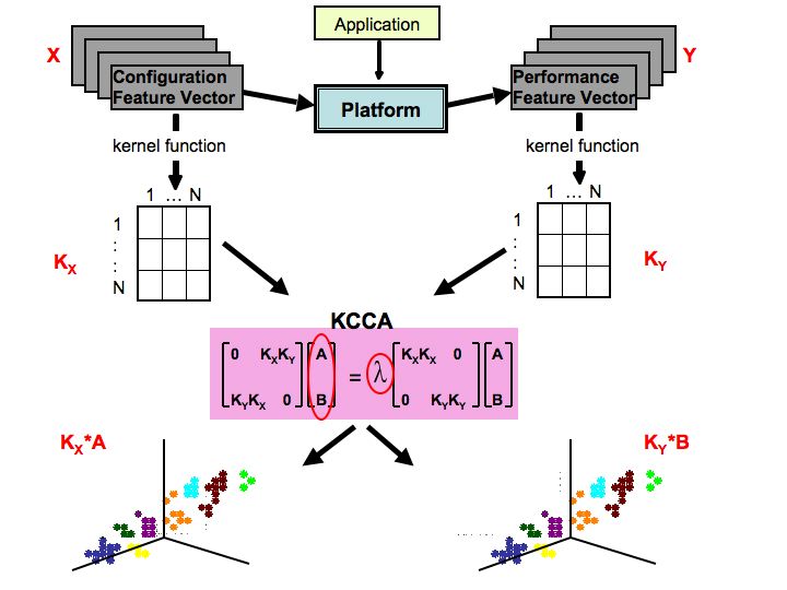
Auto-tuning in the context that we are proposing explores a much larger search space than the previous work, thereby exercising the full potential of newer SML algorithms. Recast from a SML perspective, auto-tuning leverages relationships between a set of optimization parameters and a set of resultant performance metrics to explore the search space. Kernel Canonical Correlation Analysis (KCCA) [4] is a recent SML algorithm that effectively identifies these relationships. Specifically, KCCA finds multivariate correlations between optimization parameters and performance metrics on a training set of data. We can then use these statistical relationships to optimize for performance and energy efficiency.
For the training set data, KCCA first takes the vector representations of the configuration parameters (X) and the corresponding performance metrics (Y). Next, we construct a matrix Kx that captures the similarity of each configuration vector to every other configuration vector, and a matrix Ky that compares each performance vector to every other performance vector. Given Kx and Ky , KCCA produces a matrix A of basis vectors onto which Kx can be projected, and a matrix B of basis vectors onto which Ky can be projected, such that KxA and KyB are maximally correlated. That is, neighborhoods in KxA correspond to neighborhoods in KyB . We compute matrices A and B by solving the generalized eigenvector equation shown in Figure 1.
There are several design decisions to be considered when customizing KCCA for auto-tuning:
In the following section, we present an example of optimizing a scientific code using a customized version of the KCCA algorithm.
Stencil (nearest-neigbor) computations are used extensively in partial differential equation (PDE) solvers involving structured grids [1]. In a typical stencil code, each grid point updates its value based on the values of its nearest neighbors. These neighbors define the stencil shape, which will be constant for every point in the grid.
Our work utilizes 3D 7-point and 27-point stencils arising from finite difference calculations. For each stencil run, we perform a single sweep over a grid where the read and write arrays are distinct. The 27-point stencil performs significantly more FLOPs per byte transferred than the 7-point stencil (1.25 vs. 0.33 FLOPs/byte) and thus is more likely to be compute-bound.
We conduct our experimental runs on two superscalar out-of-order machines: the Intel Clovertown and the AMD Barcelona, which Table 1 details. For each platform, we compile appropriate code variants for the 7-point and 27-point stencils. See [8] for details on each optimization and its corresponding parameters.
For each stencil, we randomly choose 1500 configurations to build our training data sets. We limit our sample size to 1500 datapoints as the KCCA algorithm is exponential with respect to the number of datapoints. We run the stencil code variant reflecting each chosen configuration and collect low-level performance counter data as detailed in Section 3.2. Then we use kernel functions (described in Section 3.3) to compare the similarity of every pair of stencil runs in our training set, generating two matrices that are input to our KCCA algorithm. KCCA projects these two matrices onto subspaces such that the projections are maximally correlated. However, by the nature of KCCA, it is difficult to reverse-engineer which features of the data contribute to a dimension of correlation. Thus we look up the projection of the best performing datapoint in our training set and use a genetic algorithm in that neighborhood, as described in Section 3.4. The result of this step is a new set of configurations that we run to find an optimal configuration.
Next, we consider several design decisions to customize KCCA for stencil code optimization.
For each stencil code run, we construct one configuration vector and one performance vector. The configuration feature vector is built using parameters for the optimizations listed in Table 2. See [8] for details. Similarly, the performance feature vector uses the counters listed in Table 3 as features and the measurements of these counters as values. We also measure Watts consumed using a power meter attached to our machines.
Using N=1500 runs per stencil, the N configuration vectors of K=16 features are combined into a N x K configuration matrix; the N performance vectors of L features (L=8 for Clovertown and L=6 for Barcelona) produce a N x L performance matrix. The corresponding rows in each of the two matrices describe the same stencil run.
Since our performance vector contains solely numeric values, we use the Gaussian kernel function [17] below:
Since the configuration vectors contain both numeric and non-numeric values, we construct a kernel function using a combination of two other kernel functions. For numeric features, we use the Gaussian kernel function. For non-numeric features we define:
Thus, given the N x K configuration matrix and the N x L performance matrix, we form a N x N matrix Kx and a N x N matrix Ky , which are used as input to the KCCA algorithm.
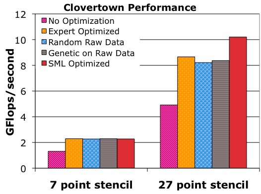
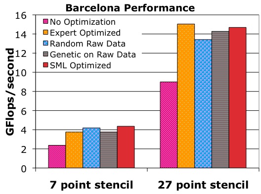
Note that the clock rate is 2.66 GHz for Clovertown and 2.30 GHz for Barcelona. Furthermore, the number of FLOPs per point is 8 for the 7-point stencil and 30 for the 27-point stencil. Figures 2(a) and 2(b) show a breakdown of the GFLOP rate our SML methodology achieves for Clovertown and Barcelona respectively. They also compare our results to the no-optimization configuration and an expert optimized configuration [8].
On Clovertown, our technique provides performance within .02 GFLOPs/sec (1%) of expert optimized for the 7-point stencil and 1.5 GFLOPs/sec (18%) better for the 27-point stencil. Because the 7-point stencil is bandwidth bound on the Clovertown, none of the techniques show significant performance gains. The significant performance gain for the 27-point can be attributed to two factors: (i) our domain decomposition parameters more efficiently exploit the 27-point stencil's data locality; (ii) we likely use registers and functional units more efficiently as a result of our inner loop parameter values.
On Barcelona, our performance is 0.6 GFLOPs/sec (16%) better than that achieved by expert optimized for the 7-point stencil and within 0.35 GFLOPs/sec (2%) for the 27-point stencil. For the 7-point stencil, our inner loop optimization parameters unroll along a different dimension than expert optimized. We also prefetch further ahead than the expert optimized configuration. For the 27-point stencil on Barcelona, the dominant factor causing the performance gap is the smaller padding size in the unit stride dimension used by the expert optimized configuration. Furthermore, the expert's configuration use more efficient domain decomposition.
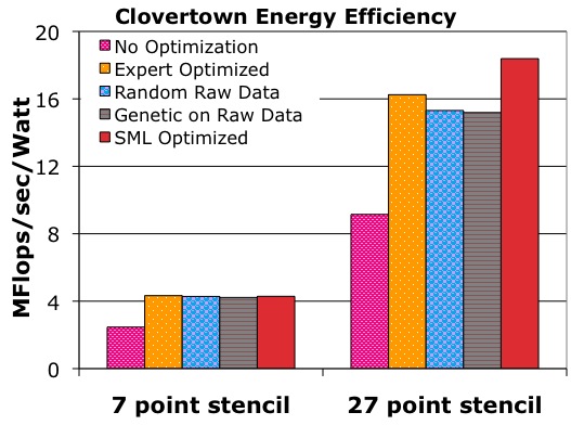
The second metric of success is energy efficiency. Based on power meter wattage readings, we calculate energy efficiency with the following formula:
As seen in Figure 2(c), on Clovertown we achieve within 1% of the expert optimized energy efficiency for the 7-point stencil and 13% better than expert optimized for the 27-point stencil. For both our stencil codes on Clovertown and the 27-point stencil code on Barcelona, the best performing configuration is also the most energy efficient. For the 7-point stencil on Barcelona, the energy efficiency of our fastest run differs from the most energy efficient run by a mere 0.3%. As a result, we have omitted the Barcelona energy efficiency graph.
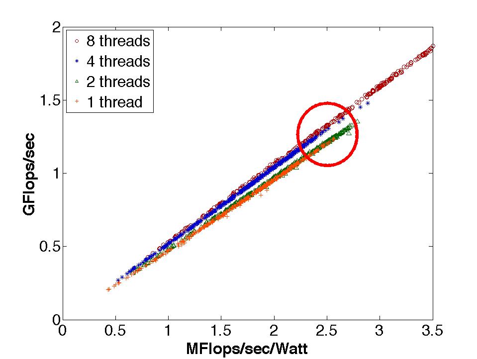
Figure 2(d) compares performance against energy efficiency on the Clovertown. The slope of the graph represents Watts consumed, and since marker shape/color denote thread count, we see that power consumption is dictated by the number of threads used. We observe configurations with identical performance but differing energy efficiency and vice versa, as highlighted by the red oval. In environments with real-time constraints (e.g., portable devices), there is no benefit to completing well before the real-time deadline; but there is significant benefit to conserving battery power. In such environments, performance can be sacrificed for energy efficiency, and thus we expect a wider gap between the two metrics.
|
For instance, the Roofline model considers memory bandwidth as a potential bottleneck. Considering only compulsory misses in our stencil codes, we achieve 95.4% of Stream bandwidth for the 7-point stencil and 13.8% more than the Stream bandwidth for the 27-point stencil on the Clovertown platform. We exceed Stream bandwidth for the 27-point stencil because the Stream benchmark is unoptimized. On Barcelona, we achieve 89.2% of Stream bandwidth for the 7-point stencil and 80.1% for the 27-point stencil. Since Barcelona has a lower FLOP to byte ratio than Clovertown, the stencils are more likely to be compute bound on this platform. As a result, we are unable to achieve a higher fraction of stream bandwidth.
We have shown that SML can quickly identify configurations that simultaneously optimize running time and energy efficiency. SML based auto-tuning methodologies are agnostic to the underlying architecture as well as the code being optimized, resulting in a scalable alternative to human expert-optimization.
As an example, we optimized two stencil codes on two multicore architectures, either matching or outperforming a human expert by up to 18%. The optimization process took about two hours to explore a space that would take half a year to explore exhaustively on a single computer by conventional techniques. This result gives us reason to believe that SML effectively handles the combinatorial explosion posed by the optimization parameters, potentially allowing us to explore some previously-intractable research directions:
Our results to date, and the promise of mapping difficult research problems such as those above onto approaches similar to our own, give us confidence that SML will open up exciting new opportunities to advance the state-of-the-art in multicore performance optimization.
0.97
 (a)
(a)
 (b)
(b)
 (c)
(c)
 (d)
(d)