
| Paper | Description | Used to measure |
| HAC [17] | File system with 17000 files totaling 150 MB | Time and space needed to create a Glimpse index |
| IRON [36] | None provided | Checksum and metadata replication overhead; parity block overhead for user files |
| LBFS [30] | 10702 files from /usr/local, total size 354 MB | Performance of LBFS chunking algorithm |
| LISFS [34] | 633 MP3 files, 860 program files, 11502 man pages | Disk space overhead; performance of search-like activities: UNIX find and LISFS lookup |
| PAST [40] | 2 million files, mean size 86 KB, median 4 KB, largest file size 2.7 GB, smallest 0 Bytes, total size 166.6 GB | File insertion, global storage utilization in a P2P system |
| Pastiche [9] | File system with 1641 files, 109 dirs, 13.4 MB total size | Performance of backup and restore utilities |
| Pergamum [47] | Randomly generated files of ``several'' megabytes | Data transfer performance |
| Samsara [10] | File system with 1676 files and 13 MB total size | Data transfer and querying performance, load during querying |
| Segank [46] | 5-deep directory tree, 5 subdirs and 10 8 KB files per directory | Performance of Segank: volume update, creation of read-only snapshot, read from new snapshot |
| SFS read-only [15] | 1000 files distributed evenly across 10 directories and contain random data | Single client/single server read performance |
| TFS [7] | Files taken from /usr to get ``realistic'' mix of file sizes | Performance with varying contribution of space from local file systems |
| WAFL backup [20] | 188 GB and 129 GB volumes taken from the Engineering department | Performance of physical and logical backup, and recovery strategies |
| yFS [49] | Avg. file size 16 KB, avg. number of files per directory 64, random file names | Performance under various benchmarks (file creation, deletion) |
File system benchmarking is in a state of disarray. In spite of tremendous advances in file system design, the approaches for benchmarking still lag far behind. The goal of benchmarking is to understand how the system under evaluation will perform under real-world conditions and how it compares to other systems; however, recreating real-world conditions for the purposes of benchmarking file systems has proven challenging. The two main challenges in achieving this goal are generating representative workloads, and creating realistic file-system state.
While creating representative workloads is not an entirely solved problem, significant steps have been taken towards this goal. Empirical studies of file-system access patterns [4,19,33] and file-system activity traces [38,45] have led to work on synthetic workload generators [2,14] and methods for trace replay [3,26].
The second, and perhaps more difficult challenge, is to recreate the file-system state such that it is representative of the target usage scenario. Several factors contribute to file-system state, important amongst them are the in-memory state (contents of the buffer cache), the on-disk state (disk layout and fragmentation) and the characteristics of the file-system image (files and directories belonging to the namespace and file contents).
One well understood contributor to state is the in-memory state of the file system. Previous work has shown that the contents of the cache can have significant impact on the performance results [11]. Therefore, system initialization during benchmarking typically consists of a cache ``warm-up'' phase wherein the workload is run for some time prior to the actual measurement phase. Another important factor is the on-disk state of the file system, or the degree of fragmentation; it is a measure of how the disk blocks belonging to the file system are laid out on disk. Previous work has shown that fragmentation can adversely affect performance of a file system [44]. Thus, prior to benchmarking, a file system should undergo aging by replaying a workload similar to that experienced by a real file system over a period of time [44].
Surprisingly, one key contributor to file-system state has been largely ignored - the characteristics of the file-system image. The properties of file-system metadata and the actual content within the files are key contributors to file-system state, and can have a significant impact on the performance of a system. Properties of file-system metadata includes information on how directories are organized in the file-system namespace, how files are organized into directories, and the distributions for various file attributes such as size, depth, and extension type. Consider a simple example: the time taken for a find operation to traverse a file system while searching for a file name depends on a number of attributes of the file-system image, including the depth of the file-system tree and the total number of files. Similarly, the time taken for a grep operation to search for a keyword also depends on the type of files (i.e., binary vs. others) and the file content.
File-system benchmarking frequently requires this sort of information on file systems, much of which is available in the form of empirical studies of file-system contents [1,12,21,29,41,42]. These studies focus on measuring and modeling different aspects of file-system metadata by collecting snapshots of file-system images from real machines. The studies range from a few machines to tens of thousands of machines across different operating systems and usage environments. Collecting and analyzing this data provides useful information on how file systems are used in real operating conditions.
In spite of the wealth of information available in file-system studies, system designers and evaluators continue to rely on ad hoc assumptions and often inaccurate rules of thumb. Table 1 presents evidence to confirm this hypothesis; it contains a (partial) list of publications from top-tier systems conferences in the last ten years that required a test file-system image for evaluation. We present both the description of the file-system image provided in the paper and the intended goal of the evaluation.
In the table, there are several examples where a new file system or application design is evaluated on the evaluator's personal file system without describing its properties in sufficient detail for it to be reproduced [7,20,36]. In others, the description is limited to coarse-grained measures such as the total file-system size and the number of files, even though other file-system attributes (e.g., tree depth) are relevant to measuring performance or storage space overheads [9,10,17,30]. File systems are also sometimes generated with parameters chosen randomly [47,49], or chosen without explanation of the significance of the values [15,34,46]. Occasionally, the parameters are specified in greater detail [40], but not enough to recreate the original file system.
The important lesson to be learnt here is that there is no standard technique to systematically include information on file-system images for experimentation. For this reason, we find that more often than not, the choices made are arbitrary, suited for ease-of-use more than accuracy and completeness. Furthermore, the lack of standardization and reproducibility of these choices makes it near-impossible to compare results with other systems.
To address these problems and improve one important aspect of file system benchmarking, we develop Impressions, a framework to generate representative and statistically accurate file-system images. Impressions gives the user flexibility to specify one or more parameters from a detailed list of file system parameters (file-system size, number of files, distribution of file sizes, etc.). Impressions incorporates statistical techniques (automatic curve-fitting, resolving multiple constraints, interpolation and extrapolation, etc.) and uses statistical tests for goodness-of-fit to ensure the accuracy of the image.
We believe Impressions will be of great use to system designers, evaluators, and users alike. A casual user looking to create a representative file-system image without worrying about carefully selecting parameters can simply run Impressions with its default settings; Impressions will use pre-specified distributions from file-system studies to create a representative image. A more sophisticated user has the power to individually control the knobs for a comprehensive set of file-system parameters; Impressions will carefully work out the statistical details to produce a consistent and accurate image. In both cases, Impressions ensures complete reproducibility of the image, by reporting the used distributions, parameter values, and seeds for random number generators.
In this paper we present the design, implementation and evaluation of the Impressions framework (§3), which we intend to release for public use in the near future. Impressions is built with the following design goals:
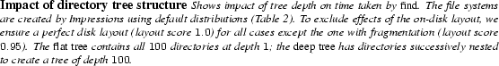
Structure and organization of file-system metadata matters for workload performance. Let us take a look at the simple example of a frequently used UNIX utility: find. Figure 1 shows the relative time taken to run ``find /'' searching for a file name on a test file system as we vary some parameters of file-system state.
The first bar represents the time taken for the run on the original
test file system.
Subsequent bars are normalized to this time and show performance for a run
with the file-system contents in buffer cache,
a fragmented version of the same file system, a file system created by
lattening the original directory tree, and finally one by deepening the
original directory tree.
The graph echoes our understanding of caching and fragmentation, and brings
out one aspect that is often overlooked: structure really matters.
From this graph we can see that even for a simple workload, the impact
of tree depth on performance can be as large as that with fragmentation,
and varying tree depths can have significant performance variations
(![]() between the flat and deep trees in this example).
between the flat and deep trees in this example).
Assumptions about file-system structure have often trickled into file system design, but no means exist to incorporate the effects of realistic file-system images in a systematic fashion. As a community, we well understand that caching matters, and have begun to pay attention to fragmentation, but when it comes to file-system structure, our approach is surprisingly laissez faire.
We believe that the file-system image used for an evaluation should be realistic with respect to the workload; the image should contain a sufficient degree of detail to realistically exercise the workload under consideration. An increasing degree of detail will likely require more effort and slow down the process. Thus it is useful to know the degree sufficient for a given evaluation. For example, if the performance of an application simply depends on the size of files in the file system, the chosen file-system image should reflect that. On the other hand, if the performance is also sensitive to the fraction of binary files amongst all files (e.g., to evaluate desktop search indexing), then the file-system image also needs to contain realistic distributions of file extensions.
We walk through some examples that illustrate the different degrees of detail needed in file-system images.
Impressions is designed with this goal of flexibility from the outset. The user is given complete control of a number of file-system parameters, and is provided with an easy to use interface. Transparently, Impressions seamlessly ensures accuracy and representativeness.
One alternate approach to generating realistic file-system images is to randomly select a set of actual images from a corpus, an approach popular in other fields of computer science such as Information Retrieval, Machine Learning and Natural Language Processing [32]. In the case of file systems the corpus would consist of a set of known file-system images (e.g., tarballs). This approach arguably has several limitations which make it difficult and unsuitable for file systems research. First, there are too many parameters required to accurately describe a file-system image that need to be captured in a corpus. Second, without precise control in varying these parameters according to experimental needs, the evaluation can be blind to the actual performance dependencies. Finally, the cost of maintaining and sharing any realistic corpus of file-system images would be prohibitive. The size of the corpus itself would severely restrict its usefulness especially as file systems continue to grow larger.
Unfortunately, these limitations have not deterred researchers from using their personal file systems as a (trivial) substitute for a file-system corpus.
In this section we describe the design, implementation and evaluation of Impressions: a framework for generating file-system images with realistic and statistically accurate metadata and content . Impressions is flexible enough to create file-system images with varying configurations, guaranteeing the accuracy of images by incorporating a number of statistical tests and techniques.
We first present a summary of the different modes of operation of Impressions, and then describe the individual statistical constructs in greater detail. Wherever applicable, we evaluate their accuracy and performance.
| Parameter | Default Model & Parameters |
| Directory count w/ depth | Generative model |
| Directory size (subdirs) | Generative model |
| File size by count | Lognormal-body |
| (
|
|
| Pareto-tail (k= |
|
| File size by containing | Mixture-of-lognormals |
| bytes | (
|
|
|
|
| Extension popularity | Percentile values |
| File count w/ depth | Poisson ( |
| Bytes with depth | Mean file size values |
| Directory size (files) | Inverse-polynomial |
| (degree= |
|
| File count w/ depth | Conditional probabilities |
| (w/ special directories) | (biases for special dirs) |
| Degree of Fragmentation | Layout score (1.0) |
| or Pre-specified workload |
A system evaluator can use Impressions in different modes of operation, with varying degree of user input.
Sometimes, an evaluator just wants to create a representative file-system image without worrying about the need to carefully select parameters. Hence, in the automated mode, Impressions is capable of generating a file-system image with minimal input required from the user (e.g., the size of the desired file-system image), relying on default settings of known empirical distributions to generate representative file-system images. We refer to these distributions as original distributions.
At other times, users want more control over the images, for example, to analyze the sensitivity of performance to a given file-system parameter, or to describe a completely different file-system usage scenario. Hence, Impressions supports a user-specified mode, where a more sophisticated user has the power to individually control the knobs for a comprehensive set of file-system parameters; we refer to these as user-specified distributions. Impressions carefully works out the statistical details to produce a consistent and accurate image.
In both the cases, Impressions ensures complete reproducibility of the file-system image by reporting the used distributions, their parameter values, and seeds for random number generators.
Impressions can use any dataset or set of parameterized curves for the original distributions, leveraging a large body of research on analyzing file-system properties [1,12,21,29,41,42].
For illustration, in this paper we use a recent
static file-system snapshot dataset made publicly
available [1].
The snapshots of file-system metadata were collected over a five-year period
representing over ![]() Windows PC file systems in a large corporation.
These snapshots were used to study distributions and temporal changes in
file size, file age,
file-type frequency, directory size, namespace structure, file-system
population, storage capacity, and degree of file
modification. The study also proposed a generative model explaining the
creation of file-system namespaces.
Windows PC file systems in a large corporation.
These snapshots were used to study distributions and temporal changes in
file size, file age,
file-type frequency, directory size, namespace structure, file-system
population, storage capacity, and degree of file
modification. The study also proposed a generative model explaining the
creation of file-system namespaces.
Impressions provides a comprehensive set of individually controllable file system parameters. Table 2 lists these parameters along with their default selections. For example, a user may specify the size of the file-system image, the number of files in the file system, and the distribution of file sizes, while selecting default settings for all other distributions. In this case, Impressions will ensure that the resulting file-system image adheres to the default distributions while maintaining the user-specified invariants.
The goal of Impressions is to generate realistic file-system images, giving the user complete flexibility and control to decide the extent of accuracy and detail. To achieve this, Impressions relies on a number of statistical techniques.
In the simplest case, Impressions needs to create statistically accurate file-system images with default distributions. Hence, a basic functionality required by Impressions is to convert the parameterized distributions into real sample values used to create an instance of a file-system image. Impressions uses random sampling to take a number of independent observations from the respective probability distributions. Wherever applicable, such parameterized distributions provide a highly compact and easy-to-reproduce representation of observed distributions. For cases where standard probability distributions are infeasible, a Monte Carlo method is used.
A user may want to use file system datasets other than the default choice. To enable this, Impressions provides automatic curve-fitting of empirical data.
Impressions also provides the user with the flexibility to specify distributions and constraints on parameter values. One challenge thus is to ensure that multiple constraints specified by the user are resolved consistently. This requires statistical techniques to ensure that the generated file-system images are accurate with respect to both the user-specified constraints and the default distributions.
In addition, the user may want to explore values of file system parameters, not captured in any dataset. For this purpose, Impressions provides support for interpolation and extrapolation of new curves from existing datasets.
Finally, to ensure the accuracy of the generated image, Impressions contains a number of built-in statistical tests, for goodness-of-fit (e.g., Kolmogorov-Smirnov, Chi-Square, and Anderson-Darling), and to estimate error (e.g., Confidence Intervals, MDCC, and Standard Error). Where applicable, these tests ensure that all curve-fit approximations and internal statistical transformations adhere to the highest degree of statistical rigor desired.
The simplest use of Impressions is to generate file-system images with realistic metadata. This process is performed in two phases: first, the skeletal file-system namespace is created; and second, the namespace is populated with files conforming to a number of file and directory distributions.
The first phase in creating a file system is to create the namespace structure or the directory tree. We assume that the user specifies the size of the file-system image. The count of files and directories is then selected based on the file system size (if not specified by the user). Depending on the degree of detail desired by the user, each file or directory attribute is selected step by step until all attributes have been assigned values. We now describe this process assuming the highest degree of detail.
To create directory trees, Impressions uses the generative model
proposed by Agrawal et al. [1] to perform a
Monte Carlo simulation.
According to this model, new directories are added to a file
system one at a time, and the probability of choosing
each extant directory as a parent is proportional
to
![]() , where
, where
![]() is the count of extant subdirectories of directory
is the count of extant subdirectories of directory ![]() .
The model explains the creation of the file system namespace,
accounting both for the size and count of
directories by depth, and the size of parent directories. The
input to this model is the total number of directories
in the file system. Directory names are generated using a simple
iterative counter.
.
The model explains the creation of the file system namespace,
accounting both for the size and count of
directories by depth, and the size of parent directories. The
input to this model is the total number of directories
in the file system. Directory names are generated using a simple
iterative counter.
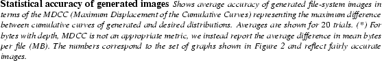
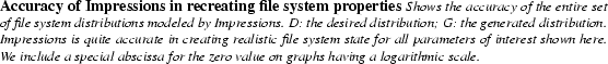
To ensure the accuracy of generated images, we compare the generated distributions (i.e., created using the parameters listed in Table 2), with the desired distributions (i.e., ones obtained from the dataset discussed previously in §3.1). Figure 2 shows in detail the accuracy for each step in the namespace and file creation process. For almost all the graphs, the y-axis represents the percentage of files, directories, or bytes belonging to the categories or bins shown on the x-axis, as the case may be.
Figures 2(a) and 2(b) show the distribution of directories by depth, and directories by subdirectory count, respectively. The y-axis in this case is the percentage of directories at each level of depth in the namespace, shown on the x-axis. The two curves representing the generated and the desired distributions match quite well, indicating good accuracy and reaffirming prior results [1].
The next phase is to populate the directory tree with files. Impressions spends most of the total runtime and effort during this phase, as the bulk of its statistical machinery is exercised in creating files. Each file has a number of attributes such as its size, depth in the directory tree, parent directory, and file extension. Similarly, the choice of the parent directory is governed by directory attributes such as the count of contained subdirectories, the count of contained files, and the depth of the parent directory. Analytical approximations for file system distributions proposed previously [12] guided our own models.
First, for each file,
the size of the file is sampled from a hybrid distribution
describing file sizes. The body of this hybrid curve is approximated
by a lognormal distribution, with a Pareto tail distribution
(k=![]() ,
,
![]() =512MB)
accounting for the heavy tail of files with size greater than
512 MB.
The exact parameter values used for these distributions are
listed in Table 2. These parameters
were obtained by fitting the respective curves to file sizes
obtained from the file-system dataset previously discussed (§3.1).
Figure 2(c) shows the accuracy of generating
the distribution of files by size.
We initially used a simpler model for file sizes represented
solely by a lognormal distribution. While the results were
acceptable for files by size
(Figure 2(c)), the simpler model failed
to account for the distribution of bytes by containing
file size; coming up with a model to accurately capture the bimodal distribution of bytes
proved harder than we had anticipated.
Figure 2(d) shows the accuracy of the
hybrid model in Impressions in generating the distribution of bytes.
The pronounced double mode observed in the
distribution of bytes is a result of the presence of a few large files;
an important detail that is otherwise missed if the heavy-tail
of file sizes is not accurately accounted for.
=512MB)
accounting for the heavy tail of files with size greater than
512 MB.
The exact parameter values used for these distributions are
listed in Table 2. These parameters
were obtained by fitting the respective curves to file sizes
obtained from the file-system dataset previously discussed (§3.1).
Figure 2(c) shows the accuracy of generating
the distribution of files by size.
We initially used a simpler model for file sizes represented
solely by a lognormal distribution. While the results were
acceptable for files by size
(Figure 2(c)), the simpler model failed
to account for the distribution of bytes by containing
file size; coming up with a model to accurately capture the bimodal distribution of bytes
proved harder than we had anticipated.
Figure 2(d) shows the accuracy of the
hybrid model in Impressions in generating the distribution of bytes.
The pronounced double mode observed in the
distribution of bytes is a result of the presence of a few large files;
an important detail that is otherwise missed if the heavy-tail
of file sizes is not accurately accounted for.
Once the file size is selected, we assign the file name and
extension. Impressions keeps a list of percentile values for popular file extensions
(i.e., top ![]() extensions by count, and by bytes).
These extensions together account for roughly 50% of
files and bytes in a file system ensuring adequate coverage
for the important extensions. The remainder of files are
given randomly generated three-character extensions. Currently
filenames are generated by a simple numeric counter incremented on
each file creation.
Figure 2(e) shows the accuracy of Impressions in
creating files with popular extensions by count.
extensions by count, and by bytes).
These extensions together account for roughly 50% of
files and bytes in a file system ensuring adequate coverage
for the important extensions. The remainder of files are
given randomly generated three-character extensions. Currently
filenames are generated by a simple numeric counter incremented on
each file creation.
Figure 2(e) shows the accuracy of Impressions in
creating files with popular extensions by count.
Next, we assign file depth ![]() , which requires satisfying two
criteria: the
distribution of files with depth, and the distribution of bytes
with depth. The former is modeled by a Poisson distribution,
and the latter is represented by the mean file sizes at a given
depth. Impressions uses a multiplicative model combining the two criteria,
to produce appropriate file depths. Figures 2(f)
and 2(g) show the accuracy in generating the
distribution of files by depth, and the distribution of bytes by
depth, respectively.
, which requires satisfying two
criteria: the
distribution of files with depth, and the distribution of bytes
with depth. The former is modeled by a Poisson distribution,
and the latter is represented by the mean file sizes at a given
depth. Impressions uses a multiplicative model combining the two criteria,
to produce appropriate file depths. Figures 2(f)
and 2(g) show the accuracy in generating the
distribution of files by depth, and the distribution of bytes by
depth, respectively.
The final step is to select a parent directory for the file, located at
depth ![]() ,
according to the distribution of
directories with file count, modeled using an inverse-polynomial of degree
,
according to the distribution of
directories with file count, modeled using an inverse-polynomial of degree ![]() .
As an added feature, Impressions supports the notion of ``Special'' directories
containing a disproportionate number of files or bytes
(e.g., ``Program Files'' folder in the Windows
environment). If required, during the selection of the parent directory,
a selection bias is given to these special directories.
Figure 2(h) shows the accuracy in supporting
special directories with an example of a typical Windows file system
having files in the web cache at depth
.
As an added feature, Impressions supports the notion of ``Special'' directories
containing a disproportionate number of files or bytes
(e.g., ``Program Files'' folder in the Windows
environment). If required, during the selection of the parent directory,
a selection bias is given to these special directories.
Figure 2(h) shows the accuracy in supporting
special directories with an example of a typical Windows file system
having files in the web cache at depth ![]() , in
Windows and Program Files folders at depth
, in
Windows and Program Files folders at depth ![]() , and
System files at depth
, and
System files at depth ![]() .
.
| Parameter | MDCC |
| Directory count with depth | 0.03 |
| Directory size (subdirectories) | 0.004 |
| File size by count | 0.04 |
| File size by containing bytes | 0.02 |
| Extension popularity | 0.03 |
| File count with depth | 0.05 |
| Bytes with depth | 0.12 MB* |
| File count w/ depth w/ special dirs | 0.06 |
| Num. files | Sum of file sizes | File size distribution | Avg. |
Avg. |
Avg. |
Avg. D | Avg. D | Success |
|
|
|
|
Initial | Final | Count | Bytes | ||
| 1000 | 30000 | ( |
21.55% | 2.04% | 5.74% | 0.043 | 0.050 | 100% |
| 1000 | 60000 | ( |
20.01% | 3.11% | 4.89% | 0.032 | 0.033 | 100% |
| 1000 | 90000 | ( |
34.35% | 4.00% | 41.2% | 0.067 | 0.084 | 90% |
Multiple constraints can also be implicit (i.e., arise even in the
absence of user-specified distributions).
Due to random sampling, different sample sets of the same distribution are not
guaranteed to produce exactly the same result, and consequently, the sum of the
elements can also differ across samples. Consider the previous example of file sizes again: the sum of all file
sizes drawn from a given distribution need not add up to the desired
file system size (total used space) each time.
More formally, this example is represented by the following set of
constraints:
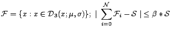

The problem of resolving multiple constraints as formulated above, is a
variant of the more general ``Subset Sum Problem''
which is NP-complete [8].
Our solution is thus an approximation algorithm based
on an existing
![]() solution [37]
for the Subset Sum Problem.
solution [37]
for the Subset Sum Problem.
The existing algorithm has two phases. The first phase randomly chooses a solution vector which is valid (the sum of elements is less than the desired sum), and maximal (adding any element not already in the solution vector will cause the sum to exceed the desired sum). The second phase performs local improvement: for each element in the solution, it searches for the largest element not in the current solution which, if replaced with the current element, would reduce the difference between the desired and current sums. The solution vector is updated if such an element is found, and the algorithm proceeds with the next element, until all elements are compared.
Our problem definition and the modified algorithm differ from the original in the following ways:
Consider an example where a user has specified a desired
file system size of ![]() bytes, a lognormal file size distribution
(
bytes, a lognormal file size distribution
(![]() =
=![]() ,
, ![]() =
=![]() ), and
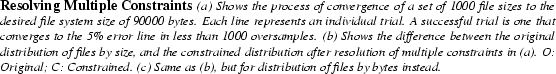
), and ![]() files. Figure 3(a) shows the convergence
of the sum of file sizes in a sample set obtained with this distribution.
Each line in the graph represents an independent trial,
starting at a y-axis value equal to the sum of its initially sampled file sizes.
Note that in this example, the initial sum differs from the desired sum
by more than a 100% in several cases.
The x-axis represents the number of extra iterations (oversamples)
performed by the algorithm. For a trial to succeed, the sum of file sizes
in the sample must converge to within 5% of the desired file system size.
We find that in most cases
files. Figure 3(a) shows the convergence
of the sum of file sizes in a sample set obtained with this distribution.
Each line in the graph represents an independent trial,
starting at a y-axis value equal to the sum of its initially sampled file sizes.
Note that in this example, the initial sum differs from the desired sum
by more than a 100% in several cases.
The x-axis represents the number of extra iterations (oversamples)
performed by the algorithm. For a trial to succeed, the sum of file sizes
in the sample must converge to within 5% of the desired file system size.
We find that in most cases ![]() ranges between 0 and
ranges between 0 and ![]() (i.e., less than
(i.e., less than ![]() oversampling); and in almost all cases,
oversampling); and in almost all cases,
![]() .
.
The distribution of file sizes in
![]() must be close
to the original distribution in
must be close
to the original distribution in
![]() .
Figure 3(b) and 3(c)
show the difference between the original and constrained distributions for file
sizes (for files by size, and files by bytes),
for one successful trial from Figure 3(a).
We choose these particular distributions as examples throughout this paper
for two reasons.
First, file size is an important parameter, so we want to be particularly thorough
in its accuracy. Second, getting an accurate shape for the bimodal curve of
files by bytes presents a challenge for Impressions; once we get our techniques
to work for this curve, we are fairly confident of its accuracy on simpler
distributions.
.
Figure 3(b) and 3(c)
show the difference between the original and constrained distributions for file
sizes (for files by size, and files by bytes),
for one successful trial from Figure 3(a).
We choose these particular distributions as examples throughout this paper
for two reasons.
First, file size is an important parameter, so we want to be particularly thorough
in its accuracy. Second, getting an accurate shape for the bimodal curve of
files by bytes presents a challenge for Impressions; once we get our techniques
to work for this curve, we are fairly confident of its accuracy on simpler
distributions.
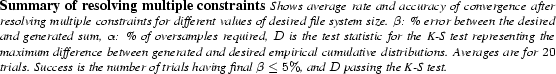
We find that Impressions resolves multiple constraints to satisfy
the requirement on the sum, while respecting the original distributions.
Table 4 gives the summary for the above
example of file sizes for different values of the desired file system size.
The expected sum of ![]() file sizes, sampled as specified in the table,
is close to
file sizes, sampled as specified in the table,
is close to ![]() . Impressions successfully converges the initial
sample set to the desired sum with an average oversampling rate
. Impressions successfully converges the initial
sample set to the desired sum with an average oversampling rate ![]() less
than 5%. The average difference between the desired and achieved sum
less
than 5%. The average difference between the desired and achieved sum
![]() is close to 3%. The constrained distribution passes the two-sample K-S
test at the
is close to 3%. The constrained distribution passes the two-sample K-S
test at the ![]() significance level, with the difference between the two
distributions being fairly small (the
significance level, with the difference between the two
distributions being fairly small (the ![]() statistic of the K-S test is around 0.03,
which represents the maximum difference between two
empirical cumulative distributions).
statistic of the K-S test is around 0.03,
which represents the maximum difference between two
empirical cumulative distributions).
We repeat the above experiment for two more choices of file system sizes,
one lower than the expected mean (30K), and one higher (90K);
we find that even when the desired sum is quite different from the
expected sum, our algorithm performs well.
Only for ![]() of the
of the ![]() trials in the 90K case,
did the algorithm fail to converge. For these extreme cases, we drop the initial sample and start over.
trials in the 90K case,
did the algorithm fail to converge. For these extreme cases, we drop the initial sample and start over.
Impressions requires knowledge of the distribution of file system parameters necessary to create a valid image. While it is tempting to imagine that Impressions has perfect knowledge about the nature of these distributions for all possible values and combinations of individual parameters, it is often impossible.
First, the empirical data is limited to what is observed in any given dataset and may not cover the entire range of possible values for all parameters. Second, even with an exhaustive dataset, the user may want to explore regions of parameter values for which no data point exists, especially for ``what if'' style of analysis. Third, from an implementation perspective, it is more efficient to maintain compact representations of distributions for a few sample points, instead of large sets of data. Finally, if the empirical data is statistically insignificant, especially for outlying regions, it may not serve as an accurate representation. Impressions thus provides the capability for interpolation and extrapolation from available data and distributions.
Impressions needs to generate complete new curves from existing ones. To illustrate our procedure, we describe an example of creating an interpolated curve; extensions to extrapolation are straightforward. Figure 4 shows how Impressions uses piece-wise interpolation for the distribution of files with containing bytes. In this example, we start with the distribution of file sizes for file systems of size 10 GB, 50 GB and 100 GB, shown in the figure. Each power-of-two bin on the x-axis is treated as an individual segment, and the available data points within each segment are used as input for piece-wise interpolation; the process is repeated for all segments of the curve. Impressions combines the individual interpolated segments to obtain the complete interpolated curve.
| Distribution | FS Region | D | K-S Test |
| (I/E) | Statistic | ( |
|
| File sizes by count | 75GB (I) | 0.054 | passed |
| File sizes by count | 125GB (E) | 0.081 | passed |
| File sizes by bytes | 75GB (I) | 0.105 | passed |
| File sizes by bytes | 125GB (E) | 0.105 | passed |
Actual file content can have substantial impact on the performance of an application. For example, Postmark [24], one of the most popular file system benchmarks, tries to simulate an email workload, yet it pays scant attention to the organization of the file system, and is completely oblivious of the file data. Postmark fills all the ``email'' files with the same data, generated using the same random seed. The evaluation results can range from misleading to completely inaccurate, for instance in the case of content-addressable storage (CAS). When evaluating a CAS-based system, the disk-block traffic and the corresponding performance will depend only on the unique content - in this case belonging to the largest file in the file system. Similarly, performance of Desktop Search and Word Processing applications is sensitive to file content.
In order to generate representative file content, Impressions supports a number of options. For human-readable files such as .txt, .html files, it can populate file content with random permutations of symbols and words, or with more sophisticated word-popularity models. Impressions maintains a list of the relative popularity of the most popular words in the English language, and a Monte Carlo simulation generates words for file content according to this model. However, the distribution of word popularity is heavy-tailed; hence, maintaining an exhaustive list of words slows down content generation. To improve performance, we use a word-length frequency model [43] to generate the long tail of words, and use the word-popularity model for the body alone. The user has the flexibility to select either one of the models in entirety, or a specific combination of the two. It is also relatively straightforward to add extensions in the future to generate more nuanced file content. An example of such an extension is one that carefully controls the degree of content similarity across files.
In order to generate content for typed files, Impressions either contains enough information to generate valid file headers and footers itself, or calls into a third-party library or software such as Id3v2 [31] for mp3; GraphApp [18] for gif, jpeg and other image files; Mplayer [28] for mpeg and other video files; asciidoc for html; and ascii2pdf for PDF files.
To isolate the effects of file system content,
Impressions can measure the degree of
on-disk fragmentation, and create file systems with user-defined
degree of fragmentation.
The extent of fragmentation is measured in terms of
layout score [44]. A layout score
of ![]() means all files in the file system are laid out optimally
on disk (i.e., all blocks of any given file are laid out consecutively
one after the other), while a layout score of 0 means that no two blocks
of any file are adjacent to each other on disk.
means all files in the file system are laid out optimally
on disk (i.e., all blocks of any given file are laid out consecutively
one after the other), while a layout score of 0 means that no two blocks
of any file are adjacent to each other on disk.
Impressions achieves the desired degree of fragmentation by issuing pairs of temporary file create and delete operations, during creation of regular files. When experimenting with a file-system image, Impressions gives the user complete control to specify the overall layout score. In order to determine the on-disk layout of files, we rely on the information provided by debugfs. Thus currently we support layout measurement only for Ext2 and Ext3. In future work, we will consider several alternatives for retrieving file layout information across a wider range of file systems. On Linux, the FIBMAP and FIEMAP ioctl()s are available to map a logical block to a physical block [23]. Other file system-specific methods exist, such as the XFS_IOC_GETBMAP ioctl for XFS.
The previous approach however does not account for differences in fragmentation strategies across file systems. Impressions supports an alternate specification for the degree of fragmentation wherein it runs a pre-specified workload and reports the resulting layout score. Thus if a file system employs better strategies to avoid fragmentation, it is reflected in the final layout score after running the fragmentation workload.
There are several alternate techniques for inducing more realistic fragmentation in file systems. Factors such as burstiness of I/O traffic, out-of-order writes and inter-file layout are currently not accounted for; a companion tool to Impressions for carefully creating fragmented file systems will thus be a good candidate for future research.
| Time taken (seconds) | ||
| FS distribution (Default) | ||
| Directory structure | 1.18 | 1.26 |
| File sizes distribution | 0.10 | 0.28 |
| Popular extensions | 0.05 | 0.13 |
| File with depth | 0.064 | 0.29 |
| File and bytes with depth | 0.25 | 0.70 |
| File content (Single-word) | 0.53 | 1.44 |
| On-disk file/dir creation | 437.80 | 1394.84 |
| Total time | 473.20 | 1826.12 |
| (8 mins) | (30 mins) | |
| File content (Hybrid model) | 791.20 | - |
|
Layout score ( |
133.96 | - |

| App | Parameter & Value | Comment on Validity |
| GDL | File content |
10% of files and 5% of bytes |
| (content in deeper namespace is growing) | ||
| GDL | Text file sizes |
13% of files and 90% of bytes |
| Beagle | Text file cutoff |
0.13% of files and 71% of bytes |
| Beagle | Archive files |
4% of files and 84% of bytes |
| Beagle | Shell scripts |
20% of files and 89% of bytes |
![\includegraphics[width=2.1in, height=1.25in]{graphs/eps/bgl-gdl-txtword-size.eps}](img108.png)
|
![\includegraphics[width=2.1in]{graphs/content-usenix/eps/beagle-newmedia.eps}](img109.png)
![\includegraphics[width=2.1in]{graphs/content-usenix/eps/beagle-newmedia-space.eps}](img110.png)
|
In this section, we use Impressions to evaluate desktop searching applications. Our goals for this case study are two-fold. First, we show how simple it is to use Impressions to create either representative images or images across which a single parameter is varied. Second, we show how future evaluations should report the settings of Impressions so that results can be easily reproduced.
We choose desktop search for our case study because its performance
and storage requirements depend not only on the file system size and
structure, but also on the type of files and the actual content within
the files. We evaluate two desktop search applications:
open-source Beagle [5] and Google's Desktop for Linux (GDL) [16].
Beagle supports a large number of file types using ![]() search-filters;
it provides several indexing options,
trading performance and index size with the quality and
feature-richness of the index. Google Desktop does not provide as
many options: a web interface allows users to select or exclude
types of files and folder locations for searching, but does
not provide any control over the type and quality of indexing.
search-filters;
it provides several indexing options,
trading performance and index size with the quality and
feature-richness of the index. Google Desktop does not provide as
many options: a web interface allows users to select or exclude
types of files and folder locations for searching, but does
not provide any control over the type and quality of indexing.
Developers of data-intensive applications frequently need to make assumptions about the properties of file-system images. For example, file systems and applications can often be optimized if they know properties such as the relative proportion of meta-data to data in representative file systems. Previously, developers could infer these numbers from published papers [1,12,41,42], but only with considerable effort. With Impressions, developers can simply create a sample of representative images and directly measure the properties of interest.
Table 6 lists assumptions we found in GDL and Beagle limiting the search indexing to partial regions of the file system. However, for the representative file systems in our data set, these assumptions omit large portions of the file system. For example, GDL limits its index to only those files less than ten directories deep; our analysis of typical file systems indicates that this restriction causes 10% of all files to be missed. We believe that instead of arbitrarily specifying hard values, application designers should experiment with Impressions to find acceptable choices.
We note that Impressions is useful for discovering these application assumptions and for isolating performance anomalies that depend on the file-system image. Isolating the impact of different file systems feature is easy using Impressions: evaluators can use Impressions to create file-system images in which only a single parameter is varied, while all other characteristics are carefully controlled.
This type of discovery is clearly useful when one is using
closed-source code, such as GDL. For example, we discovered the GDL
limitations by constructing file-system images across which a single
parameter is varied (e.g., file depth and file size), measuring the
percentage of indexed files, and noticing precipitous drops in this
percentage. This type of controlled experimentation is also useful
for finding non-obvious performance interactions in open-source code.
For instance, Beagle uses the inotify mechanism [22] to
track each directory for change; since the default Linux kernel
provides ![]() watches, Beagle resorts to manually crawling the
directories once their count exceeds
watches, Beagle resorts to manually crawling the
directories once their count exceeds ![]() . This deterioration in
performance can be easily found by creating file-system images with
varying numbers of directories.
. This deterioration in
performance can be easily found by creating file-system images with
varying numbers of directories.
The time spent by desktop search applications to crawl a file-system image is significant (i.e., hours to days); therefore, it is likely that different developers will innovate in this area. In order for developers to be able to compare their results, they must be able to ensure they are using the same file-system images. Impressions allows one to precisely control the image and report the parameters so that the exact same image can be reproduced.
For desktop search, the type of files (i.e., their extensions) and the content of files has a significant impact on the time to build the index and its size. We imagine a scenario in which the Beagle and GDL developers wish to compare index sizes. To make a meaningful comparison, the developers must clearly specify the file-system image used; this can be done easily with Impressions by reporting the size of the image, the distributions listed in Table 2, the word model, disk layout, and the random seed. We anticipate that most benchmarking will be done using mostly default values, reducing the number of Impressions parameters that must be specified.
An example of the reporting needed for reproducible results is shown in Figure 7. In these experiments, all distributions of the file system are kept constant, but only either text files (containing either a single word or with the default word model) or binary files are created. These experiments illustrate the point that file content significantly affects the index size; if two systems are compared using different file content, obviously the results are meaningless. Specifically, different file types change even the relative ordering of index size between Beagle and GDL: given text files, Beagle creates a larger index; given binary files, GDL creates a larger index.
Figures 8 gives an additional example of reporting Impressions parameters to make results reproducible. In these experiments, we discuss a scenario in which different developers have optimized Beagle and wish to meaningfully compare their results. In this scenario, the original Beagle developers reported results for four different images: the default, one with only text files, one with only image files, and one with only binary files. Other developers later create variants of Beagle: TextCache to display a small portion of every file alongside a search hit, DisDir to disable directory indexing, and DisFilter to index only attributes. Given the reported Impressions parameters, the variants of Beagle can be meaningfully compared to one another.
In summary, Impressions makes it extremely easy to create both controlled and representative file-system images. Through this brief case study evaluating desktop search applications, we have shown some of the advantages of using Impressions. First, Impressions enables developers to tune their systems to the file system characteristics likely to be found in their target user populations. Second, it enables developers to easily create images where one parameter is varied and all others are carefully controlled; this allows one to assess the impact of a single parameter. Finally, Impressions enables different developers to ensure they are all comparing the same image; by reporting Impressions parameters, one can ensure that benchmarking results are reproducible.
We discuss previous research in four areas related to file system benchmarking and usage of file system metadata.
First, Impressions enables file system measurement studies to be put into practice. Besides the metadata studies on Windows workstations [1,12], previous work in non-Windows environment includes Satyanarayanan's study of a Digital PDP-10 [41], Irlam's and Mullender's studies of Unix systems [21,29], and the study of HP-UX systems at Hewlett-Packard [42]. These studies provide valuable data for designers of file systems and related software, and can be easily incorporated in Impressions.
Second, several models have been proposed to explain observed file-system phenomena. Mitzenmacher proposed a generative model, called the Recursive Forest File model [27] to explain the behavior of file size distributions. The model accounts for the hybrid distribution of file sizes with a lognormal body and Pareto tail. Downey's Multiplicative File Size model [13] is based on the assumption that new files are created by using older files as templates e.g., by copying, editing or filtering an old file. The size of the new file in this model is given by the size of the old file multiplied by an independent factor. These models provide an intuitive understanding of the underlying phenomena, and are also easier for computer simulation. In future, Impressions can be enhanced by incorporating more such models.
Third, a number of tools and techniques have been proposed to improve the state of the art of benchmarking. Chen and Patterson proposed a ``self-scaling'' benchmark that scales with the I/O system being evaluated, to stress the system in meaningful ways [6]. TBBT is a NFS trace replay tool that derives the file-system image underlying a trace [50]. It extracts the file system hierarchy from a given trace in depth-first order and uses that during initialization for a subsequent trace replay. While this ensures a consistent file-system image for replay, it does not solve the more general problem of creating accurately controlled images for all types of file system benchmarking. The Auto-Pilot tool [48] provides an infrastructure for running tests and analysis tools to automate the benchmarking process.
Finally, workload is an important piece of the benchmarking puzzle. The SynRGen file reference generator by Ebling and Satyanarayan [14] generates synthetic equivalents for real file system users. The volumes or images in their work make use of simplistic assumptions about the file system distributions as their focus is on user access patterns. Roselli et al. collected dynamic file system usage patterns in UNIX and Windows NT environments and studied file system access behavior [39]. Recent work on file system workloads includes a study of network file system usage at NetApp [25].
File system benchmarking is in a state of disarray. One key aspect of this problem is generating realistic file-system state, with due emphasis given to file-system metadata and file content. To address this problem, we develop Impressions, a statistical framework to generate realistic and configurable file-system images. Impressions provides the user flexibility in selecting a comprehensive set of file system parameters, while seamlessly ensuring accuracy of the underlying images, serving as a useful platform for benchmarking.
In our experience, we find Impressions easy to use and well suited for a number of tasks. It enables application developers to tune their systems to the file system characteristics likely found in their target users. Impressions also makes it feasible to compare performance of systems by standardizing and reporting all used parameters, a requirement necessary for benchmarking. We believe Impressions will prove to be a valuable tool for system developers and users alike; we intend to release it for public use in the near future. Please check https://www.cs.wisc.edu/adsl/Software/Impressions/to obtain a copy.
We are grateful to Bill Bolosky for providing us with a copy of the five-year metadata dataset from Microsoft. Lakshmi Bairavasundaram provided many useful discussions and gave valuable comments on earlier drafts of this paper. Finally, we would like to thank Valerie Aurora Henson (our shepherd) and the anonymous reviewers for their excellent feedback and comments.
This material is based upon work supported by the National Science Foundation under the following grants: CCF-0621487, CNS-0509474, as well as by generous donations from Network Appliance and Sun Microsystems. Any opinions, findings, and conclusions or recommendations expressed in this material are those of the authors and do not necessarily reflect the views of NSF or other institutions.
This document was generated using the LaTeX2HTML translator Version 2002-2-1 (1.70)
Copyright © 1993, 1994, 1995, 1996,
Nikos Drakos,
Computer Based Learning Unit, University of Leeds.
Copyright © 1997, 1998, 1999,
Ross Moore,
Mathematics Department, Macquarie University, Sydney.
The command line arguments were:
latex2html -split 0 -show_section_numbers -local_icons -no_navigation -white main.tex
The translation was initiated by Nitin Agrawal on 2009-01-15

![\includegraphics[width=2.2in]{graphs/basic/eps/depth-dir.eps}](img48.png)
![\includegraphics[width=2.2in]{graphs/basic/eps/countsubdirs.eps}](img49.png)
![\includegraphics[width=2.2in]{graphs/basic/eps/sizebycount.eps}](img50.png)
![\includegraphics[width=2.2in]{graphs/basic/eps/sizebybytes-pareto.eps}](img51.png)
![\includegraphics[width=2.2in]{graphs/basic/eps/topextensioncount.eps}](img52.png)
![\includegraphics[width=2.2in]{graphs/basic/eps/depth-files.eps}](img53.png)
![\includegraphics[width=2.2in]{graphs/basic/eps/depth-meanbytes.eps}](img54.png)
![\includegraphics[width=2.2in]{graphs/basic/eps/depth-files-specialdir.eps}](img55.png)
![\includegraphics[width=2.2in]{graphs/multiconstraint/eps/multicons-converge-1000.eps}](img61.png)
![\includegraphics[width=2.2in]{graphs/multiconstraint/eps/multi-count.eps}](img62.png)
![\includegraphics[width=2.2in]{graphs/multiconstraint/eps/multi-bytes.eps}](img63.png)
![\includegraphics[width=2.7in]{graphs/interpolate/piecewise-interpolation.eps}](img90.png)
![\includegraphics[width=1.6in]{graphs/interpolate/eps/int-75-count.eps}](img92.png)
![\includegraphics[width=1.6in]{graphs/interpolate/eps/int-75-bytes.eps}](img93.png)
![\includegraphics[width=1.6in]{graphs/interpolate/eps/ext-125-count.eps}](img94.png)
![\includegraphics[width=1.6in]{graphs/interpolate/eps/ext-125-bytes.eps}](img95.png)