SWEEPER: An Efficient Disaster Recovery Point Identification
Mechanism
| Akshat Verma |
Kaladhar Voruganti |
Ramani Routray |
Rohit Jain 1 |
| IBM India Research |
Network Appliance |
IBM Almaden Research |
Yahoo India |
| akshatverma@in.ibm.com |
kaladhar.voruganti@netapp.com |
routrayr@us.ibm.com |
rohitj@yahoo-inc.com
|
Abstract:
Data corruption is one of the key problems that is on top of the radar
screen of most CIOs. Continuous Data Protection (CDP) technologies help
enterprises deal with data corruption by maintaining multiple versions of data
and facilitating recovery by allowing an administrator restore to an earlier
clean version of data. The aim of the recovery process after data corruption is
to quickly traverse through the backup copies (old versions), and retrieve a
clean copy of data. Currently, data recovery is an ad-hoc, time consuming and
frustrating process with sequential brute force approaches, where recovery time
is proportional to the number of backup copies examined and the time to check a
backup copy for data corruption.
In this paper, we present the design and implementation of SWEEPER
architecture and backup copy selection algorithms that specifically tackle the
problem of quickly and systematically identifying a good recovery point. We
monitor various system events and generate checkpoint records that help in
quickly identifying a clean backup copy. The SWEEPER methodology
dynamically determines the selection algorithm based on user specified recovery
time and recovery point objectives, and thus, allows system administrators to
perform trade-offs between recovery time and data currentness. We have
implemented our solution as part of a popular Storage Resource Manager product
and evaluated SWEEPER under many diverse settings. Our study clearly
establishes the effectiveness of SWEEPER as a robust strategy to
significantly reduce recovery time.
1
Introduction
Data Resiliency is a very important concern for most organizations to ensure
business continuity in the face of different types of failures and disasters,
such as virus attacks, site failures, machine/firmware malfunction, accidental
and malicious human/application errors [17,2].
Resiliency is not only about being able to resurrect data after failures, but
also about how quickly the data can be resurrected so that the business can be
operational again. While in the case of total data loss failures, the recovery
time is largely dominated by Restoration Cost, i.e., time to restore
the data from backup systems at local or remote locations; in the case of data
corruption failures, the time to identify a clean previous copy of data to
revert to can be much larger. Often, data corruption is detected after the
incidence of corruption itself. As a result, the administrator has a large
number of candidate backup copies to select the recovery point from. The key to
fast recovery in such cases is reducing the time required in the identification
step. Much research and industrial attention have been devoted to protecting
data from disasters. However, relatively little work has been done in the area
of how to quickly retrieve the latest clean copy of uncorrupted data. The focus
of this paper is on how to efficiently identify clean data.
Data resiliency is based on Data Protection: taking either
continuous or periodic snapshots of the data as it is being updated. Block level
[7]
[15],
file level [10],
logical volume level [27]
and database level [5]
data replication/recovery mechanisms are the most prominent data protection
mechanisms. The mechanisms vary with respect to their support for different data
granularities, transactional support, replication site distance, backup
latencies, recovery point and recovery time objectives [11].
Continuous data protection (CDP) [24] is a
form of continuous data protection that allows one to go back in time after a
failure and recover earlier versions of an object at the granularity of a single
update.
The recovery process is preceded by Error Detection. Errors are
usually found either by application users or by automated data integrity tools.
Tools such as disk scrubbers and S.M.A.R.T. tools [23] can
detect corruptions caused by hardware errors. Virus scanners, application
specific data integrity checkers such as fsck for filesystem integrity, and
storage level intrusion detection tools [19,3]
can detect logical data corruptions caused by malicious software, improper
system shutdown, and erroneous administrator actions. For complex Storage Area
Network (SAN) environments, configuration validation tools [1]
have been proposed that can be used in both proactive and reactive mode to
identify configuration settings that could potentially lead to logical data
corruptions.
Once system administrators are notified of a corruption, they need to solve
the Recovery Point Identification problem, i.e., determine a recovery
point that will provide a clean copy of their data. Typically, system
administrators choose a recovery point by trading-off recovery speed (the number
of versions that need to be checked to find a clean copy) versus data
currentness (one might not want to lose valid data updates for the sake of fast
recovery). Recovery point identification is currently a manual, error-prone and
frustrating process for system administrators, due to the pressure to quickly
bring organization's applications back on-line. Even though CDP technologies
provide users with the ability to rollback every data update, they do not
address the problem of identifying a clean copy of data. It is only after a good
recovery point has been identified, that Data Recovery can begin by
replacing the corrupt copy by the clean copy of data. The efficacy of a recovery
process is characterized by a Recovery Time Objective (RTO) and a Recovery Point
objective (RPO). RTO measures the downtime after detection of corruption,
whereas RPO indicates the loss in data currency in terms of seconds of updates
that are lost.
This paper describes and evaluates methods for efficient recovery point
identification in CDP logs which reduce RTO, while not compromising on RPO. The
basic idea behind our approach is to evaluate the events generated by various
components such as applications, file systems, databases and other
hardware/software resources and generate checkpoint records. Subsequently upon
the detection of failure, we efficiently process these checkpoint records to
start the recovery process from an appropriate CDP record. Since CDP mechanisms
are typically used along with point-in-time snapshot (PIT) technologies, it is
possible to create data copies selectively. Further, since the time it takes to
test a copy of data for corruption dominates overall recovery time, selective
testing of copies can drastically reduce recovery time. This selective
identification of copies that one can target for quick recovery is the focus of
this work.
Some existing CDP solutions [16,21,30] are
based on the similar idea of checkpointing interesting events in CDP
logs. While event checkpointing mechanisms help in narrowing down the search
space, they do not guarantee that the most appropriate checkpoint record will be
identified. Thus, the CDP log evaluation techniques presented in this paper
compliment these checkpoint record generation mechanisms in quickly identifying
the most suitable CDP record. The key contributions of this paper are:
- SWEEPER Recovery Point Identification Architecture: We
present the architecture of an extensible recovery point identification tool
that consists of event monitoring, checkpoint generation, clean copy detection
and CDP log processing components. The architectural framework is independent
of specific applications and can easily be used with other application
specific CDP solutions such as [16,21].
- Novel Event Checkpointing Mechanism: Data corruptions are usually
not silent but are accompanied by alerts and warning messages from
applications, file systems, operating systems, SAN elements (e.g., switches,
virtualization engines), storage controllers and disks. Table 2
lists some events that usually accompany data corruption caused by various
components. We define a mechanism that identifies events from various
application and system activities and uses a combination of a) expert provided
knowledge base, b) resource dependency analysis, and c) a event correlation
technique to correlate them with various types of corruption.
- CDP Record Scanning Algorithms: We present three different CDP
record scanning algorithms that efficiently process the event checkpoints for
identifying the appropriate CDP log record for data recovery. The scanning
mechanisms isolate a recovery point quickly by using the observations that (a)
pruning the space of timestamps into equal sized partitions reduces the search
space exponentially and (b) checkpoint records that have high correlation with
corruptions are more likely to be indicative of corruption. One of the novel
features of the checkpoint record selection process is the acceptance of
recovery time objective (RTO) and recovery point objective (RPO) as input
parameters. Thus, the algorithms have the desirable property of providing a
tradeoff between the total execution time and the data currency at the
recovery point. The expected execution time of the algorithms is logarithmic
in the number of checkpoint records examined and linear in the number of data
versions tested for integrity. The proposed algorithms are robust with noise
in the checkpoint record generation process, and can deal with errors in
correlation probability estimation. Further, even though they are not designed
to deal with silent errors, they still find a recovery point in logarithmic
time for silent errors.
- Performance Evaluation: We present an implementation of the
SWEEPER architecture and algorithms in context of a popular Storage
Resource Manager product (IBM Total Storage Productivity Center), and
demonstrate the scalability of our design. We also present a comparative
analysis of the various Record Scanning algorithms proposed by us under
different operational parameters, which include failure correlation
probability distribution for events, number of checkpoint records, and rate of
false negatives. We identify the different scenarios for which each algorithm
is most suited and conclusively establish the efficacy of the SWEEPER
methodology.
The rest of this paper is organized as follows. We formally define the
Recovery Point Identification problem and model in Sec. 2.1
and 2.2.
The SWEEPER architecture is presented in Sec. 2.3.
The CDP record scanning algorithms are described in Sec.3, and
our implementation in Sec. 4.
Sec. 5
describes our experimental evaluation. Sec. 6
discusses the strengths and weaknesses of SWEEPER in the context of
related work followed by a conclusion in Sec. 7.
We now provide a formal definition of the Recovery
Point Identification problem and model parameters.
2.1
Problem Formulation
We investigate the problem of data recovery after a
failure has resulted in data corruption. Data corruption is detected by an
integrity checker (possibly with application support). The second step in this
process is to identify the nature of corruption (e.g., virus corruption,
hardware error). For isolating the problem, the components (e.g, controllers,
disks, switches, applications) that may be the cause of error are identified by
constructing a mapping from the corrupted data to the applications. Once the
affected components are identified, the recovery module finds a time instance to
go back to when the data was uncorrupted. Once the time instance is identified,
CDP logs and point-in-time images are used to construct the uncorrupted data.
Table 1: Notations
 |
Time at which data was last
known to be clean |
 |
Time at which corruption was
detected |
 |
Timestamp  |
 |
Error Timestamp |
 |
Number of CDP logs after which a
PIT copy is taken |
 |
Number of CDP logs between and |
 |
Number of checkpoints between
and |
 |
Time taken for recovery |
 |
Cost of getting a PIT copy
online and ready to read/write |
 |
Average Cost of applying one CDP
log entry |
 |
Cost of testing one data image
for corruption |
 |
probability that checkpoint  is correlated with corruption is correlated with corruption | |
We now formally describe the Recovery Point Identification
problem. The notations used in this paper are tabulated in Table. 1.
The Recovery Point Identification problem is to minimize the total time
taken to recover the data in order to get the most current uncorrupted data
(i.e., find a timestamp such that  while minimizing
). A constrained version of the problem is to minimize
while minimizing
). A constrained version of the problem is to minimize  subject to a bound on . The identification of proceeds by finding
an ordered set
subject to a bound on . The identification of proceeds by finding
an ordered set  of timestamps, which is a subset of the set of all the
timestamps
of timestamps, which is a subset of the set of all the
timestamps  such that
  (
( ), the last element of the set , is the same as
the error point . Further, the total cost of creating and testing the data
images corresponding to the
), the last element of the set , is the same as
the error point . Further, the total cost of creating and testing the data
images corresponding to the  timestamps in , which equals , should be minimized. The cost of checking a data image at timestamp
for corruption is the sum of (a) the cost of making the first PIT
image preceding the timestamp available for read/write () (b) the cost of
applying the
timestamps in , which equals , should be minimized. The cost of checking a data image at timestamp
for corruption is the sum of (a) the cost of making the first PIT
image preceding the timestamp available for read/write () (b) the cost of
applying the  ( modulo ) CDP logs (
  ) and (c) the cost of testing the copy (). Hence, the total
time spent in isolating the uncorrupted copy is the sum of the costs of all the
timestamps checked in the sequence .
) and (c) the cost of testing the copy (). Hence, the total
time spent in isolating the uncorrupted copy is the sum of the costs of all the
timestamps checked in the sequence .
2.2
Recovery Point Parameters and Estimating Sequential Checking Time
Figure 1: Timeline for testing the
snapshot at time : 1 Getting a full backup online. 2 Applying
incremental backups over it. 3 Applying CDP logs to create the snapshot at
time . 4 Testing the data for integrity.
![\includegraphics[width=7.5cm]{figs/timeline.eps}](SWEEPER_files/img30.png) |
We now elaborate on the recovery parameters like , etc and
their typical values. For a typical example, consider Fig. 1,
where a Recovery Point Identification strategy decided to check data
image at for corruption. The data protection (continuous and
point-in-time) solution employed in the setting takes a total backup of the data
at regular intervals. In between total backups, incremental backups are taken
after every writes (CDP logs). The number of incremental backups
taken between two consecutive total backups is denoted by  . Hence,
in order to construct the point-in-time snapshot of data at time , we make
the first total backup copy preceding (labeled as
. Hence,
in order to construct the point-in-time snapshot of data at time , we make
the first total backup copy preceding (labeled as  in the example) online. Then, we apply incremental backups over this
data till we reach the timestamp
in the example) online. Then, we apply incremental backups over this
data till we reach the timestamp  of the last
incremental backup point before . The total time
taken in getting the PIT copy at online is denoted
by . On this PIT copy, we now apply the CDP logs that capture all the data
changes made between and , and incur a cost
of for each log. Finally, an integrity check is applied over this data,
and the running time of the integrity checker is denoted by .
of the last
incremental backup point before . The total time
taken in getting the PIT copy at online is denoted
by . On this PIT copy, we now apply the CDP logs that capture all the data
changes made between and , and incur a cost
of for each log. Finally, an integrity check is applied over this data,
and the running time of the integrity checker is denoted by .
For average metadata and data write sizes of  and
and  respectively, write coalescing factor
  , average filesize
 , read and write bandwidth of
  and
and  respectively, a file corpus of
  files, and a unit
integrity test time
files, and a unit
integrity test time  , the expected time taken for each of these three
activities are given by the following equations. ( calculation is
based on the assumption that constructing the PIT copy only requires metadata
updates.)
, the expected time taken for each of these three
activities are given by the following equations. ( calculation is
based on the assumption that constructing the PIT copy only requires metadata
updates.)
In a typical setup with  files being are
modified every second, update sizes of
files being are
modified every second, update sizes of  , file sizes of
 , metadata size of
  , total backups
every 12 hours, incremental backups every
, total backups
every 12 hours, incremental backups every  , and disk transfer
rate of
, and disk transfer
rate of  , the time taken to get a PIT image online is
approximately 50 seconds. The time taken to apply the CDP logs is of the order
of 10 minutes, whereas the I/O time taken (not including any computations) by
the integrity checker comes to about 4 hours assuming that the
integrity checker only needs to check the modified files. In a deployment with a
CDP log window of
, the time taken to get a PIT image online is
approximately 50 seconds. The time taken to apply the CDP logs is of the order
of 10 minutes, whereas the I/O time taken (not including any computations) by
the integrity checker comes to about 4 hours assuming that the
integrity checker only needs to check the modified files. In a deployment with a
CDP log window of  hrs, if one sequentially checks every
  record, the expected time to find the point of corruption would be of the order
of
record, the expected time to find the point of corruption would be of the order
of  days. Hence, sequential checking is infeasible and minimizing the time
taken by the recovery process essentially boils down to minimizing the number of
data images that are checked by recovery process.
days. Hence, sequential checking is infeasible and minimizing the time
taken by the recovery process essentially boils down to minimizing the number of
data images that are checked by recovery process.
2.3
SWEEPER Recovery Point Identification Architecture
Figure 2: SWEEPER Recovery Point
Indentification Architecture
|
|
The central idea of SWEEPER is to automatically checkpoint
important system events from various application-independent monitoring sources
as indicators of corruption failures. In contrast to earlier work [16]
that requires an administrator to manually define the events for each
application that are correlated with various corruption types, we automate the
process of creating these checkpoints and indexing them with the type and scope
of corruption along with a number that indicates the probability of the event
being correlated with the specific corruption type. We then use these
checkpoints as hints to quickly pinpoint the most recent clean copy of data. The
overall architecture of SWEEPER is described in Fig. 2
The key design question while architecting a recovery mechanism like
SWEEPER is whether to build it a) as part of a CDP system, or b) as
part of a Storage Resource Manager product like EMC Control Center, HP OpenView
or IBM TotalStorage Productivity Centre, or c) as a standalone component. We
have separated the design of algorithms and the architecture so that the
algorithms can work with any architecture and vice versa. Implementing
SWEEPER outside the CDP system allows it to be leveraged by many
different types of CDP systems. The disadvantage of this implementation is that
some CDP systems might not completely expose all of the internal system state
changes via an event mechanism. Most of this information is available from
Storage Resource Managers. Furthermore, most Storage Resource Managers have a
comprehensive monitoring and resource discovery mechanism that can be leveraged
by the Recovery module. Hence, we recommend the design choice (b) for
SWEEPER (Fig. 2),
with the following key components.
- CDP System: CDP system is essentially a data versioning system that
can generate either log records or snapshots during data updates. The Users
can retrieve snapshots using temporal queries based on timestamps, or they can
simply traverse the snapshots using a cursor returned by query. The CDP system
also allows for restoring the data in a previous copy and make it the latest
copy.
- Storage Infra-Structure: The storage infra-structure consists of
servers (hosts), switches, storage controllers (contain disks), file systems,
database systems, virtualization boxes, and security boxes. A CDP system is
also part of the storage infra-structure but we are showing it separately in
Fig. 2.
- Storage Resource Manager: Storage resource managers contain a
discovery/monitoring engine for monitoring storage infra-structure using a
combination of SNMP protocol, CIM/SMI-S protocol, proprietary agents, in-band
protocol discovery/monitoring agents, operating system event registries, proc
file systems and application generated events. Event bus is the module in the
resource manager product that subscribes to all the events and it presents
them in a consolidated manner to other event analyzer modules. The
configuration database persistently stores the storage infra-structure
configuration data, performance data, historical trends and also event data.
The configuration database purges historical and event data based on user
specified deletion policies.
- SWEEPER Event Analyzer and Checkpoint Record Generator: This module
looks at the incoming stream of event data and filters out irrelevant events.
For the relevant events, it determines the probability that the corruption may
be correlated with this event and the scope (affected components) of the
event. After the event analysis, this module generates a checkpoint record.
The SWEEPER checkpoint record store is structured into two tiers of
checkpoints. All checkpoint records generated by Event Analyzer are
included in the lower tier and the records that have a high correlation
probability with any type of corruption are promoted to the upper tier. The
tier-ing notion can be extended from
 tiers to
  tiers. However, we observed in our experimental study that
tiers are usually sufficient for reducing recovery time.
tiers. However, we observed in our experimental study that
tiers are usually sufficient for reducing recovery time.
- SWEEPER Knowledgebase: The knowledgebase consists of records with
the following fields: a) List of event identifiers b) type or reason for data
corruption c) probability of seeing an event (or a set of correlated events)
in the case of data corruption. Corruption probability is represented as low,
medium or high values because, in many cases, it is difficult for experts to
specify exact probability values.
- Problem Determination Scanners: Failure detection can be done
either manually or using an automated checking tool, SWEEPER
leverages existing failure detection systems towards this purpose. Failure
detectors also help in determining the type of failure (e.g., virus
corruption) without pinpointing the system events that caused it.
- SWEEPER Checkpoint Record Locator: The Checkpoint Record
Locator module orchestrates the overall recovery point identification
process using one of the algorithms implemented by the CDP Record
Scanner. The first task of the Checkpoint Record Locator module
is to identify a subset of the checkpoint records that pertain to the current
data corruption it is investigating. Towards this purpose, it queries the
Problem Determination Scanner for the type and scope of the current
corruption, and identifies the components that may be the cause of corruption.
It uses the information to query the checkpoint database (indexed by type and
scope) for checkpoint records that relate to the type of corruption and
pertain to the affected components and creates a Checkpoint Record
Cache for use by the CDP Record Scanner. The Checkpoint
Record Locator allows the user to specify Recovery Time Objective or RTO
(how long the user is willing to wait for the recovery process to complete)
and Recovery Point Objective or RPO ( how stale the data can be, and this is
measure as a unit of time) and uses them along with the properties of the
Checkpoint Cache to select one of the scanning algorithms implemented
by the CDP Record Scanner. It queries the CDP Record Scanner
with the Cache and scanning algorithm as input and receives a
timestamp as the answer. It then uses the CDP Recovery Module and the
Problem Determination Scanner to create and test the data according
to the timestamp and returns the answer (corrupt/clean) of the Problem
Determination Scanner to the CDP Record Scanner and receives a new
timestamp. In each iteration of the procedure, it computes the total time
taken by the Recovery Flow and if it exceeds the RTO objective, it
terminates with the most recent clean copy of the data as the recovered data.
Also, for each timestamp that is checked, it computes the RPO (distance
between the most recent clean copy and the most stale corrupt copy) and
terminates if the RPO objective is met with the most recent clean copy of the
data.
- SWEEPER CDP Record Scanner: The CDP Record Scanner
implements an interface that takes as input a scanning strategy, a Checkpoint
record, cache, a cursor (timestamp), and the integrity (corrupt or clean) of
the cursor and returns a new cursor (timestamp) to check for data integrity.
The separation of the recovery point identification algorithms from the
checkpoint database allows SWEEPER to be flexible enough to include
new search strategies in future. Also, since the search strategies are
independent of SWEEPER, they can be implemented in other recovery
point identification architectures as well.
We now
describe the Checkpoint generation flow and Fault-isolation or
Recovery flow that capture the essence of the SWEEPER architecture.
The Checkpoint Generation flow captures the generation of checkpoint
records during normal CDP system operation. The recovery process is initiated by
system administrators when they determine that data corruption has occured and
this is captured by the Fault-Isolation flow.
Checkpoint Generation Flow:
- The CDP system generates CDP records (either logs or data copies) based on
user defined policies.
- The Storage Resource Manager product monitors and aggregates various types
of system events (hardware and software failure triggers, user action triggers
etc).
- In parallel with the CDP record generation process, the SWEEPER
event analyzer module analyzes the system events and generates a checkpoint
record for each relevant event. The checkpoint records are logically
co-related with the CDP records via timestamps.
- The checkpoint record generator a) leverages the information in the expert
knowledge base b) correlates the information in the event stream and c)
traverses the configuration resource graph, to index the checkpoint record
with the scope of the event and its correlation probability with each type of
corruption.
Fault-Isolation Flow:
- The Problem Determination Scanner or a human detects that data corruption
has occured and identifies its scope and type (e.g., virus, hardware).
- A query is posed to the SWEEPER Checkpoint Record
Locator module by the system administrator with RTO and RPO as input. The
reason or type of the data corruption and its scope is also an input to the
Checkpoint Record Locator. The input information is used by the
Checkpoint Record Locator to create a list of checkpoint records that
should be examined, and the scanning algorithm to be employed.
- The SWEEPER CDP Record Scanner is invoked with the list
of checkpoint records and the scanning strategy as input. It determines the
checkpoint record that should be examined next and returns the CDP record
corresponding to it to the user.
- The user retrieves the CDP record from the CDP system and then either runs
the appropriate diagnostics or manually examines the checkpoint record to see
whether it is corrupted. This process is repeated by the user until a clean
data copy is retrieved.
3 SWEEPER
Checkpoint Log Processing Algorithms
The checkpoint log processing algorithms are implemented in the
Checkpoint Record Locator and the CDP Record Scanner modules.
The Checkpoint Record Locator iteratively queries the CDP Record
Scanner for the next checkpoint that it should verify for correctness,
whereas the CDP Record Scanner has the core intelligence for
identifying the next eligible checkpoint. The iterative flow of Checkpoint
Record Locator is presented in Fig. 3.
Figure 3: Checkpoint Record Locator
Flow
|
|
We now present the scanning algorithms that contain the core intelligence
of SWEEPER. As in Sec. 2.1,
denotes the number of CDP logs, is the cost of
testing a data image for corruption, is the cost of
getting a PIT copy online, is the cost of
applying one CDP log on a data image and is the number of
CDP logs after which a PIT image is taken. Further, we use to
denote the number of checkpoint records in the relevant history.
The Sequential Checkpoint Strategy starts from the first clean
copy of data (Fig. 4) and
applies the CDP logs in a sequential manner. However, it creates data images
only for timestamps corresponding to some checkpoint record. The implementation
of the  algorithm returns the first checkpoint record after the
given start time. Hence, the number of integrity tests that Checkpoint
Record Locator needs to perform using the scanRecordsSequential
method is proportional to the number of checkpoint records and not
on the number of CDP logs . The worst-case cost of creating the most
current clean data image by the Sequential Scanning Strategy is
algorithm returns the first checkpoint record after the
given start time. Hence, the number of integrity tests that Checkpoint
Record Locator needs to perform using the scanRecordsSequential
method is proportional to the number of checkpoint records and not
on the number of CDP logs . The worst-case cost of creating the most
current clean data image by the Sequential Scanning Strategy is  .
.
Figure 4: Search Strategies: Sequential
follows a straight path. Binary Search reduces space by half in each step,
Informed follows a strict order between probabilities, Balanced behaves in a
probability-weighted Binary Search fashion.
|
|
We
use the observation that corruption errors are not transient in nature and
hence, if data is found to be corrupt at any time , the data would
remain corrupt for all timestamp  . This order
preservation in corruption testing allows us to partition the search space
quickly. We use the intuition of binary-search algorithms that partitioning a
search space into two equal sized partitions leads one to converge to the
required point in logarithmic time steps instead of linear number of steps.
Hence, for a search space with
. This order
preservation in corruption testing allows us to partition the search space
quickly. We use the intuition of binary-search algorithms that partitioning a
search space into two equal sized partitions leads one to converge to the
required point in logarithmic time steps instead of linear number of steps.
Hence, for a search space with  checkpoints at any
given time
checkpoints at any
given time  ,
,  returns the timestamp corresponding to the
  checkpoint record
for inspection. If the data corresponding to the timestamp is corrupt, we
recursively search for corruption in the timestamps between the
checkpoint record
for inspection. If the data corresponding to the timestamp is corrupt, we
recursively search for corruption in the timestamps between the  and checkpoints. On
the other hand, if the data is clean, our inspection window is now the
timestamps between the and the
and checkpoints. On
the other hand, if the data is clean, our inspection window is now the
timestamps between the and the  checkpoint records. It is easy to see that since
the inspection window reduces by a factor of after every check,
we would complete the search in
checkpoint records. It is easy to see that since
the inspection window reduces by a factor of after every check,
we would complete the search in  steps and the
total time (expected as well as worst case) spent in recovery point
identification is given by
steps and the
total time (expected as well as worst case) spent in recovery point
identification is given by  .
.
While identifying the next timestamp to test for corruption, the Binary
Search strategy selects the next checkpoint without taking into account the
probability that the particular checkpoint was correlated with corruption. Our
next strategy, called the Informed strategy, uses the probabilities
associated with the checkpoint records to decide the next timestamp to examine.
At any given time, it figures out the checkpoint that has the
highest likelihood () of being correlated with the corruption  . Hence, for cases where data corruption is associated with a rare
event, the search may terminate in a constant number of steps (constant number
of timestamps are examined) or take upto steps in the
adversarial worst case. However, as long as the probability of a
particular checkpoint being the cause of corruption is uncorrelated with the
time of its occurrence, the search would still reduce the space exponentially
and is expected to terminate in logarithmic steps. Formally, we have the
following result for the expected running time of Informed Search.
. Hence, for cases where data corruption is associated with a rare
event, the search may terminate in a constant number of steps (constant number
of timestamps are examined) or take upto steps in the
adversarial worst case. However, as long as the probability of a
particular checkpoint being the cause of corruption is uncorrelated with the
time of its occurrence, the search would still reduce the space exponentially
and is expected to terminate in logarithmic steps. Formally, we have the
following result for the expected running time of Informed Search.
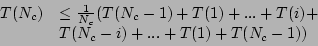
Theorem 1 The Informed
Search Strategy identifies the most recent uncorrupted data in  .
.
Proof: To prove the result, it is sufficient to prove that
the search is expected to examine only  timestamps before
it finds the most recent uncorrupted entry. It is easy to see that the average
cost of testing a given timestamp is given by
timestamps before
it finds the most recent uncorrupted entry. It is easy to see that the average
cost of testing a given timestamp is given by  .
.
Observe that as the highest probability checkpoint is uncorrelated with its
timestamp, each of the checkpoint records are equally likely to be
examined next. Further, if the  checkpoint is
examined, it divides the search space into two partitions, and we need to
examine only one of them after the check. Hence, the recurrence relation for the
search algorithm is given by
checkpoint is
examined, it divides the search space into two partitions, and we need to
examine only one of them after the check. Hence, the recurrence relation for the
search algorithm is given by
 |
(3) |
One may observe that  satisfies the recurrence relation. To verify, note that the right hand
side of the equation reduces to
satisfies the recurrence relation. To verify, note that the right hand
side of the equation reduces to  , if
, if  is replaced by
. Hence, we only need to show that
is replaced by
. Hence, we only need to show that
 for some constant
i.e., 
i.e., 
i.e., 
which holds for  by
using the fact that
by
using the fact that  . This completes the proof.
The Informed Search strategy attempts to find the corruption point
quickly by giving greater weightage to checkpoints that have a higher
correlation probability with the corruption. On the other hand, Binary
Search strategy prunes the space quickly oblivious to the probabilities
associated with the checkpoint records. We combine the key idea of both these
heuristics to design the  algorithm (Fig. 5).
The algorithm computes the total search time in an inductive manner and selects
the checkpoint record that minimizes the expected running time.
algorithm (Fig. 5).
The algorithm computes the total search time in an inductive manner and selects
the checkpoint record that minimizes the expected running time.
Figure 5: Balanced Scanning
Algorithm
|
|
Intuitively speaking, the Balanced strategy picks the checkpoint
records that (a) are likely to have caused the corruption and (b) partition the
space into two roughly equal-sized partitions. The algorithm strikes the right
balanced between partitioning the space quickly and selecting checkpoints that
are correlated with the current corruption  . We have the
following optimality result for the balanced strategy.
. We have the
following optimality result for the balanced strategy.
Theorem 2 The balanced strategy miminizes the total
expected search time required for recovery.
Proof: In order to prove the result, we formulate precisely
the expected running time of a strategy that picks a checkpoint record
for failure . The expected running time of the strategy is then given
in terms of the size and probabilities associated with the two partitions  and
and  .
.
where  and
and  are the
accumulated probabilities of the left and right partitions respectively, and
are the
accumulated probabilities of the left and right partitions respectively, and
 is the total cost of creating and testing data for any given
timestamp. Using the fact that
is the total cost of creating and testing data for any given
timestamp. Using the fact that  can be as high as
 in the case where all checkpoint records have
equal probabilities, we modify Eqn. 4
by
in the case where all checkpoint records have
equal probabilities, we modify Eqn. 4
by
Hence, the optimal strategy minimizes the term on the right hand side,
which is precisely what our balanced strategy does (after taking the common term
out from the right hand side). This completes the proof.
4
Implementation
We have implemented SWEEPER as a pluggable module
in a popular SRM (Storage Resource Manager) product, and it can use any CDP
product. We use the SRM's Event Bus to drive the checkpoint record
generation process in SWEEPER. The output of SWEEPER is a
timestamp that is fed to the CDP Recovery Module, and the
 rolls back all updates till time . Since we can
leverage many components from the SRM, the only components we needed to
implement for SWEEPER were SWEEPER Event Analyzer and Checkpoint
Generator, SWEEPER Knowledge Database, SWEEPER CDP Record
Scanner, and SWEEPER Checkpoint Record Locator. Details of the
algorithms implemented by SWEEPER CDP Record Scanner and SWEEPER
Checkpoint Record Locator have been presented in Sec. 3 and we
restrict ourselves to describing the implementation of the remaining components
in this section. We start with the checkpoint record structure and its
implementation.
In our implementation, we use a relational database to store
the checkpoint records for each event or event-set. Each checkpoint record
consists of (i) Checkpoint Record ID (ii) Timestamp
(iii)Scope (iv) Failure Type, and (v) Correlation
Probability. Checkpoint Record Id is an auto-generated primary key
and Timestamp corresponds to the time the event-set occured (consists of
year, month, day, hour, minute, second), and is synchronized with the CDP system
clock. Scope describes whether the event-set is relevant for a particular
physical device (e.g, switch, host, storage controller), or a software component
(e.g., file system, database system), or a logical construct (e.g., file, table,
zone, directory) and is used for quickly scoping the checkpoint records during
recovery. Failure Type specifies the types of failure the checkpoint is
relevant for is also used to scope the checkpoint records during recovery
processing. The failure types (hardware failure, configuration error etc) are
listed in Table 2.
Correlation Probability is computed as the probability that data
corruption happened at the same time as the occurence of the event or a set of
events.
rolls back all updates till time . Since we can
leverage many components from the SRM, the only components we needed to
implement for SWEEPER were SWEEPER Event Analyzer and Checkpoint
Generator, SWEEPER Knowledge Database, SWEEPER CDP Record
Scanner, and SWEEPER Checkpoint Record Locator. Details of the
algorithms implemented by SWEEPER CDP Record Scanner and SWEEPER
Checkpoint Record Locator have been presented in Sec. 3 and we
restrict ourselves to describing the implementation of the remaining components
in this section. We start with the checkpoint record structure and its
implementation.
In our implementation, we use a relational database to store
the checkpoint records for each event or event-set. Each checkpoint record
consists of (i) Checkpoint Record ID (ii) Timestamp
(iii)Scope (iv) Failure Type, and (v) Correlation
Probability. Checkpoint Record Id is an auto-generated primary key
and Timestamp corresponds to the time the event-set occured (consists of
year, month, day, hour, minute, second), and is synchronized with the CDP system
clock. Scope describes whether the event-set is relevant for a particular
physical device (e.g, switch, host, storage controller), or a software component
(e.g., file system, database system), or a logical construct (e.g., file, table,
zone, directory) and is used for quickly scoping the checkpoint records during
recovery. Failure Type specifies the types of failure the checkpoint is
relevant for is also used to scope the checkpoint records during recovery
processing. The failure types (hardware failure, configuration error etc) are
listed in Table 2.
Correlation Probability is computed as the probability that data
corruption happened at the same time as the occurence of the event or a set of
events.
Table 2: Monitored Events  of failure types
(): (a) Misconfiguration (b) Virus (c) Hardware related and (d)
Application, along with their monitoring source and expert information (
of failure types
(): (a) Misconfiguration (b) Virus (c) Hardware related and (d)
Application, along with their monitoring source and expert information ( )
)
![\begin{table}
\footnotesize {
\begin{minipage}[t]{.47\textwidth}
\centering {...
... High \\ \hline
\end{tabular*} \\
(d)
}
\end{minipage}
}
\end{table}](SWEEPER_files/img103.png) |
The SWEEPER checkpoint record generation centres around an
expert information repository that we call the SWEEPER Knowledge
Database. The Knowledge Database is structured as a table and a
row in the table represents an event or a set of events , and details the
source of the event, the failure type(s) relevant to the
event and the correlation probability  of the event with
each relevant failure type. A split-view of the Knowledge Base is
presented in Table 1. We use expert information derived from literature to
generate the Knowledge Database. We obtained common configuration
related probabilities from the proprietary level two field support team problem
database of a leading storage company for storage area networks. We obtained
hardware failure information from proprietary storage controller failure
database of the same company. We obtained the virus failure information by
looking at virus behavior for many common viruses at the virus encyclopedia site
[28].
To elucidate with an example, for the corruption type of virus, we looked at the
signature of the last
of the event with
each relevant failure type. A split-view of the Knowledge Base is
presented in Table 1. We use expert information derived from literature to
generate the Knowledge Database. We obtained common configuration
related probabilities from the proprietary level two field support team problem
database of a leading storage company for storage area networks. We obtained
hardware failure information from proprietary storage controller failure
database of the same company. We obtained the virus failure information by
looking at virus behavior for many common viruses at the virus encyclopedia site
[28].
To elucidate with an example, for the corruption type of virus, we looked at the
signature of the last  discovered viruses [28] and
noted common and rare events associated with them. Based on how commonly an
event is associated with a virus, we classified that event as having a low,
medium or high probability to be seen in case of a virus attack. Because of the
inherent noise in this expert data, we classify only into low, medium and high probability buckets which correspond to
probabilities of
discovered viruses [28] and
noted common and rare events associated with them. Based on how commonly an
event is associated with a virus, we classified that event as having a low,
medium or high probability to be seen in case of a virus attack. Because of the
inherent noise in this expert data, we classify only into low, medium and high probability buckets which correspond to
probabilities of  ,
,  and
and  respectively.
The events listed in the Knowledge Base and monitored by the
Event Analyzer can be classified into Configuration Changes:
addition, update (upgrade/downgrade firmware, driver or software level) or
removal of hardware and software resources and changes in security access
control. These events are checkpointed as it is common for data corruption
problems to occur when one upgrades a software level, or when one introduces a
new piece of software or hardware resource. Background Checking
Processes: successful or unsuccessful completion of background checking
processes like virus scan, hardware diagnostics, filesystem consistency like
fsck or application provided consistency checkers. These checkpoints provide
markers for consistency in specific filesystems, databases or volumes.
Application Specific Changes:Applications can provide hints about
abnormal behaviour that may indicate corruption and SWEEPER allows one
to monitor such events. Hardware Failures: checksum/CRC type errors,
self diagnostic checks like SMART, warnings generated by SMART etc.
Performance Threshold Exceeding: High port actitvity, high CPU
utilization etc. Performance Threshold Exceeding events like high port
utilization or high CPU utilization is usually a symptom of either a virus
attack, or an application that has gone astray. Meta-data Update Changes:
Changes in system directory etc. Abnormal Meta-data updates indicate
application misbehavior, which, in turn, can potentially lead to data overwrite
or corruption problems.
The  has client agents
that subscribe to various types of events from hosts, switches, storage
controllers, file systems and applications. These events are consolidated and
presented as part of an event bus. SWEEPER is only concerned about a
subset of the events in the event bus and gets the list of relevant events from
the Knowledge Database (Table 2).
Once the relevant events are filtered, the Event Analyzer generates a
checkpoint record for the event along with its timestamp. Tight synchronization
between the SWEEPER event analyzer clock and the CDP system clock is
not mandatory as the RPO granularity is no finer than
has client agents
that subscribe to various types of events from hosts, switches, storage
controllers, file systems and applications. These events are consolidated and
presented as part of an event bus. SWEEPER is only concerned about a
subset of the events in the event bus and gets the list of relevant events from
the Knowledge Database (Table 2).
Once the relevant events are filtered, the Event Analyzer generates a
checkpoint record for the event along with its timestamp. Tight synchronization
between the SWEEPER event analyzer clock and the CDP system clock is
not mandatory as the RPO granularity is no finer than  second. Hence, we
perform hourly synchronization of the event analyzer clock with the CDP clock to
ensure that the timestamps in the checkpoint records are reasonably accurate.
second. Hence, we
perform hourly synchronization of the event analyzer clock with the CDP clock to
ensure that the timestamps in the checkpoint records are reasonably accurate.
The checkpoint record scope is useful in quickly
filtering irrelevant checkpoint records, and thus, converge on the relevant CDP
records. After the initial event filtering based on the information in the
knowledgebase the checkpoint record generator examines the event type, and
determines what data (files, DB tables or volumes) can be potentially affected
by the event. We can only
Figure 6: Resource Graph
 |
determine the scope for file/DB
meta-data changes or configuration change related events. For other types of
events the notion of scope is irrelevant. The value of scope is determined by
traversing a resource graph. The resource graph information is stored in the
systems resource manager configuration database. Fig. 6 shows
a portion of the resource graph that is stored in the database. The nodes in the
graph correspond to hardware and software resources, and the edges correspond to
physical/logical connectivity or containment relationships. The basic structure
of the resource graph is the SNIA SMI-S model. However, we have made extensions
to this model to facilitate the modeling of application and database
relationships. Fig. 6
illustrates how we traverse the resource graph when a configuration changing
event occurs. If the user has added a new host and put its ports in Zone 1, then
we determine all the storage ports (and the corresponding storage controllers)
that are in zone 1. We then determine the storage volumes that are in those
storage controllers and store the ids of the storage volumes in the scope field
of the zoning event. During recovery, once the user has either manually or via
an automated tool identified a corrupt file/table/volume, we search the
checkpoint records that list the file/table/volume in its scope.
4.5
Checkpoint Record Probability Determination
Figure 7: Estimating P(e) with window
size ( ) of
) of  using Exponential-weighted Averaging
 |
The key feature of the SWEEPER
architecture is associating correlation probabilities with events to help any
search strategy in speeding up the recovery flow. For every event and
corruption , the correlation probability  denotes the probability that the corruption happened in a given
time interval given that has happened at
. The correlation probability is estimated using the Bayesian.
denotes the probability that the corruption happened in a given
time interval given that has happened at
. The correlation probability is estimated using the Bayesian.
 |
(6) |
In order to compute the correlation probability, one needs to estimate  ,
,  and . is
estimated by looking at the event stream for the event and using an
exponential-weighted averaging to compute the average frequency of the event
. To elaborate further, the time line is divided into windows of size
each (Fig. 7),
and for any window
and . is
estimated by looking at the event stream for the event and using an
exponential-weighted averaging to compute the average frequency of the event
. To elaborate further, the time line is divided into windows of size
each (Fig. 7),
and for any window  , the number of occurrences
  of
each event is noted. The local probability of event in the
window (denoted by
of
each event is noted. The local probability of event in the
window (denoted by  ) is calculated as
 . In order to take into account the historical frequency
of the event and have a more stable estimate, the probability of an
event in the time window
. In order to take into account the historical frequency
of the event and have a more stable estimate, the probability of an
event in the time window  (
( ) is
damped using the exponential decay function (Eq. 7). For
the first window, the probability is same as the local probability.
) is
damped using the exponential decay function (Eq. 7). For
the first window, the probability is same as the local probability.
 |
(7) |
The estimates are obtained from the Knowledge
Database. The final parameter in Eqn. 6 is
. However, note that whenever checkpoints are being examined to figure
out the source of a corruption , all the
checkpoints would have the same common term . Hence, is computed by ignoring the common term for
all the events, and then normalizing the correlation
probabilities so that  . The correlation
probabilities thus computed are stored in the checkpoint records for use in the
recovery flow.
. The correlation
probabilities thus computed are stored in the checkpoint records for use in the
recovery flow.
5 Evaluation
We conducted a large number of experiments to analyze the performance of
our search algorithms and study the salient features of our checkpoint-based
SWEEPER architecture. We now report some of the key findings of our
study.
Our
experimental setup is based on the implementation described in Sec. 4 and
consists of the architectural components in Fig 2.
Since real data corruption problems are relatively infrequent events, we
simulate a Fault Injector component in the interest of time. The
Fault Injector takes as input a probabilistic model of faults and its
possible signatures and generates one non-transient fault along with the
signature. Since our SWEEPER implementation is not integrated with any
CDP system, we have also simulated a CDP System Modeler and Problem
Determination Scanner. We have assumed that the Problem Determination
Scanner can accurately identify if a copy of data is corrupt or not. The
CDP System Modeler models the underlying storage and CDP system and
provides the cost and time estimates for various storage activities like the
time of applying a CDP log, making a PIT copy available for use or the time to
test a snapshot for corruption. Finally, we use an Event Generator that
mimics system activity. It takes as input a set of pre-specified events and
their distribution and generates events that are monitored by the and fed
to the SWEEPER Event Analyzer via the Event
Bus.
The key contribution of the checkpoint-based architecture is to correlate
checkpoint records with corruption failures using the correlation probabilities
. Hence, we test our search algorithms for various distributions of
, which are listed below. We use synthetic correlation probability
distributions because of the lack of authoritative traces of system and
application events that would be applicable on a wide variety of systems. We
have carefully inspected the nature of event distributions from many sources and
use the following distributions as representative distributions of
event-corruption probability.
- Uniform Distribution: This captures the setting where correlation
information between checkpoints and corruption is not known and all system
events are considered to be equally indicator of corruption.
- Zipf Distribution: The zipf distribution is commonly found in many
real-life settings and capture the adage that the probability distribution is
skewed towards a handful of events. For our experimental setting, this
captures the scenario where only a few events are the likely causes of most of
the failures.
- 2-level Uniform Distribution: A 2-level (or generally speaking a
 -level) uniform distribution has (or ) types of event-types where all the events belonging to any given
type have the same probability of having caused the corruption. However,
certain event-types are more likely to have caused the error than other
event-types and this is captured by having more than level of
probabilities.
-level) uniform distribution has (or ) types of event-types where all the events belonging to any given
type have the same probability of having caused the corruption. However,
certain event-types are more likely to have caused the error than other
event-types and this is captured by having more than level of
probabilities.
One may note that the uniform and zipf distributions capture the two extremes
in terms of skewness, that the correlation distribution may
exhibit in practice. Hence, a study with these two extreme distributions not
only capture many real settings, but also indicate the performance of the
algorithms with other distributions as well.
Our first set of experiments studied the scalability and effectiveness of the
Checkpoint Generation Flow. In the second set of experiments, we
evaluate the various search strategies in the Recovery flow. We
conducted experiments for scalability (increase in number of checkpoint records
) and their ability to deal with recovery time constraint (). We also study the usefulness of a -tier checkpoint
record structre and the robustness of the SWEEPER framework with false
negatives (probability that the error is not captured in the event stream) and
noisy data (error in correlation probability estimation). Since the CDP
system was simulated, we had to manually fix the various parameters of the
CDP system to realistic values. We kept the time taken to check the
data corresponding to any given timestamp () as  seconds, the time taken to get a PIT copy online () as
  seconds,
and the time taken to create the snapshot using the CDP logs ( ) as 100 seconds.
seconds,
and the time taken to create the snapshot using the CDP logs ( ) as 100 seconds.
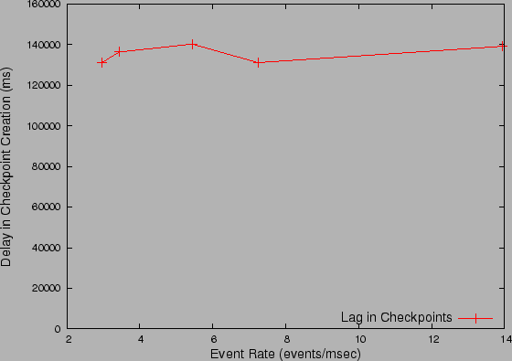
Figure 8: Lag in Checkpoint Records
with Increasing Event Rate
|
|
We first investigated the scalability of our Checkpoint Record Generation
Flow implementation to keep pace with events as the SAN size grows. Hence,
the Event Generator increases the number of resources managed by the
Storage Resource Manager and generates more events, that are fed to the
Event Analyzer. We observed that our Event Analyzer is able to
efficiently deal with increased number of events (Fig. 8) and
the lag in checkpoint record is almost independent of the event rate. We also
observe that the checkpoint records lag by only mins and hence only
the last minutes of events may be unavailable for recovery flow,
which is insignificant compared to the typical CDP windows of weeks or months
that the recovery flow has to look into. The efficiency of the checkpoint flow
is because (a) the computations in Event Analyzer (e.g.,
exponential-decay averaging) are fairly light-weight and (b) depend only on
finite-sized window (Sec. 4.5),
thus scaling well with number of events.
Figure 9: Recovery Time for Sequential
and Non-sequential strategies under Uniform probability checkpoints
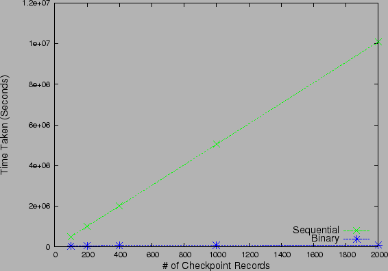 |
We next focus on the Recovery Flow and investigate the impact of
using a non-sequential strategy as opposed to sequential checking. Fig 9
compares the time taken to find the most recent uncorrupted version of data by
the sequential and the binary search strategies, for a uniform probability
distribution. Since the probability of all checkpoints are equal,
Informed as well as Balanced strategy have similar performance
to Binary Search. For the sake of visual clarity, we only plot the
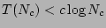
performance of Binary Search algorithm. It is clear that even for small
values of , sequential algorithm fares poorly because of the  running time ratio, and underlines the need for non-sequential
algorithms to speedup recovery. For the remainder of our experiments, we only
focus on non-sequential strategies and study their performance.
running time ratio, and underlines the need for non-sequential
algorithms to speedup recovery. For the remainder of our experiments, we only
focus on non-sequential strategies and study their performance.
Figure 10: Recovery Time for
Non-sequential strategies for (a) zipf distributed checkpoints and (b) 2-level
uniform probability checkpoints
 |
| (a) |
 |
| (b) | |
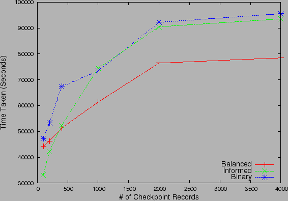
We next studied the relative performance and scalability of the proposed
non-sequential strategies for various correlation probability distributions.
Fig 10(a)
and Fig 10(b)
studies the performance of the three non-sequential strategies with increase in
the number of checkpoint records under Zipf and -level uniform
probability distribution for checkpoints. We observe that the Balanced
search strategy always outperforms the Binary search strategy.
This validates our intuition that since Balanced strategy partitions
the search space by balancing the likelihood of corruption in the partitions
rather than the number of checkpoint records it converges much faster than
binary. The gap in performance is more for the Zipf distribution than 2-level
Uniform distribution, as the more skewed Zipf distribution increases the
likelihood of partitions with equal number of checkpoints to have very different
accumulated correlation probabilities. The Informed search strategy
performs well under Zipf distribution as it has to examine very few checkpoint
records, before it identifies the recovery point. For small ,
Informed even outperforms the Balanced strategy, which takes
 time, while Informed runs in small number of
constant steps, with very high probability. Thus, if the operator has high
confidence in the events associated with different types of corruption,
Informed may be the strategy of choice. One may observe for the 2-level
uniform correlation probability case that, as the number of checkpoints
increase, the performance of Informed degrades to that of
Binary search. This is because the individual probability of each
checkpoint record (even the checkpoints associated with the higher of the
levels) falls linearly with the number of points and hence, convergence in
constant steps is no longer possible and Informed search converges in
time, while Informed runs in small number of
constant steps, with very high probability. Thus, if the operator has high
confidence in the events associated with different types of corruption,
Informed may be the strategy of choice. One may observe for the 2-level
uniform correlation probability case that, as the number of checkpoints
increase, the performance of Informed degrades to that of
Binary search. This is because the individual probability of each
checkpoint record (even the checkpoints associated with the higher of the
levels) falls linearly with the number of points and hence, convergence in
constant steps is no longer possible and Informed search converges in
 time, as predicted by Theorem 1.
These experiments bring out the fact that the greedy Informed strategy
is not good for large deployments or when the the number of backup images are
large.
time, as predicted by Theorem 1.
These experiments bring out the fact that the greedy Informed strategy
is not good for large deployments or when the the number of backup images are
large.
Figure 11: Data Currency for
Non-sequential strategies with Recovery Time Constraint under (a) 2-level
uniform distribution and (b) Zipf Distribution
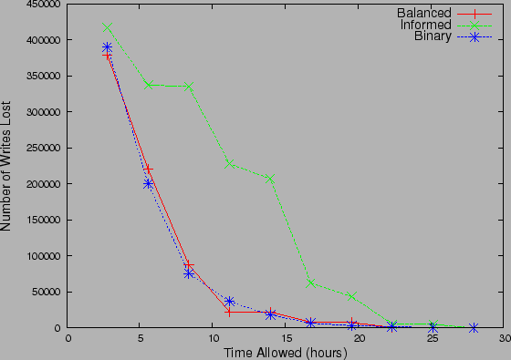 |
| (a) |
 |
| (b) | |
We next modify the objective of the search algorithms. Instead of finding the
most recent clean datapoint, the recovery algorithms now have a constraint on
the recovery time and need to output a datapoint, at the end of the time window.
Fig 11(a)
and Fig 11(b)
examine the tradeoff between the recovery execution time and the data currency
at the recovery point for 2-level uniform and Zipf distributions respectively.
Data currency is measured in terms of lost write updates between the most recent
uncorrupted copy and the copy returned by the algorithms.
The largest difference in performance under the two distribution is for the
Informed strategy. It performs well under Zipf, since it starts its
search by focusing on the few high probability checkpoints to quickly prune the
search space. Under 2-level uniform distribution, it performs poorly as compared
to the other strategies overall but more so when recovery time is less. This is
because it evaluates the uniform probability events in a random order, which on
an average leads to more unbalanced partitions, as compared to the other two
strategies. Intuitively, both the Binary and Balanced
strategies aim to reduce the unexplored space in each iteration. Hence, they
minimize the distance of the error snapshot from the set of snapshots checked by
them. On the other hand, Informed does not care about leaving a large
space unexplored by it, and hence before it finds the actual error times, its
best estimate of error time may be way off the actual error time. A similar
observation can be made if the algorithms aim to achieve a certain (non-zero)
data-currency in the minimum time possible. By reversing the axis of
Fig. 11,
one can observe that both Binary and Balanced strategies
achieve significant reduction in data-currency fairly quickly, even though
Informed catches up with them in the end. Hence, when the recovery time
window is small, the use of Informed strategy is not advisable.
Figure 12: Recovery Time for
Non-sequential strategies with 2-tier architecture
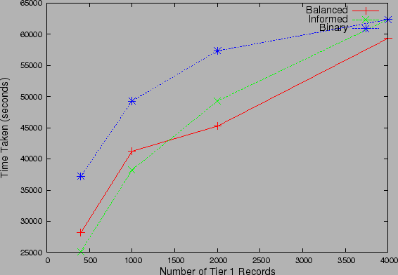 |
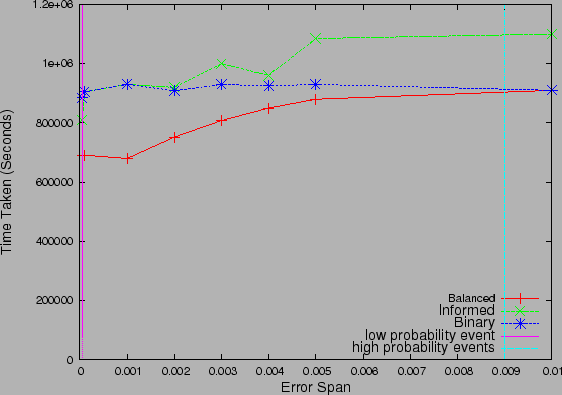
We next investigate the impact of using
a -tiered checkpoint record structure on the performance of the
algorithms. In a -tiered record structure, the algorithms execute on only a
subset of checkpoint records consisting of high probability checkpoint records.
The idea is that the recovery point is identified approximately by running the
algorithms on the smaller set of records and then locate the exact recovery
point using the checkpoints in the neighborhood. For the plot in Fig 12,
checkpoints are assigned probabilities according to 2-level uniform distribution
with  of checkpoints having
  cumulative
probability. Further, only
cumulative
probability. Further, only  of total
checkpoints are promoted to the high probability tier, and hence the skew in the
high-tier checkpoints is much lower than a single tier checkpoint record
structure. We observe in Fig. 12
that, as compared to a single tier checkpoint records (Fig 10(b)),
the performance gap between binary and balanced reduces significantly. This is
because the binary strategy reaps the benefit of operating only on the high
probability checkpoint subset, making it closer in spirit to the balanced
strategy. Thus, a -tiered checkpoint architecture, makes the probability
oblivious Binary Search algorithm also probability-aware, by forcing it
to operate only on checkpoints that have a high correlation probability with the
corruption.
of total
checkpoints are promoted to the high probability tier, and hence the skew in the
high-tier checkpoints is much lower than a single tier checkpoint record
structure. We observe in Fig. 12
that, as compared to a single tier checkpoint records (Fig 10(b)),
the performance gap between binary and balanced reduces significantly. This is
because the binary strategy reaps the benefit of operating only on the high
probability checkpoint subset, making it closer in spirit to the balanced
strategy. Thus, a -tiered checkpoint architecture, makes the probability
oblivious Binary Search algorithm also probability-aware, by forcing it
to operate only on checkpoints that have a high correlation probability with the
corruption.
Figure 13: Data Currency Loss for
Non-sequential strategies with Probability of False Negatives
 |
We next investigate the robustness of our proposed algorithms to deal with
silent errors; i.e. an error that does not generate any events. We model silent
errors using false negatives (probability that the error is not captured in the
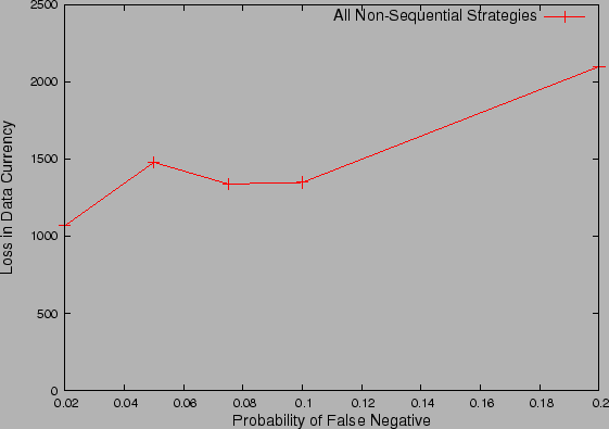
checkpoint records). Fig. 13
studies the loss in data currency with increase in false negatives. For this
experiment, the average number of CDP logs between any two events was kept at
 , and we find that the non-sequential strategies are able to keep the
data currency loss below or near this number even for a false negative of
, and we find that the non-sequential strategies are able to keep the
data currency loss below or near this number even for a false negative of  . Our results show the correlation probability-aware algorithms like
Balanced and Informed are no worse than correlation
proabibility-unaware algorithms like Sequential and Binary.
Hence, even though these strategies factor the correlation probability while
searching, they do not face significant performance penalty, when the error
event is not captured in the checkpoints.
. Our results show the correlation probability-aware algorithms like
Balanced and Informed are no worse than correlation
proabibility-unaware algorithms like Sequential and Binary.
Hence, even though these strategies factor the correlation probability while
searching, they do not face significant performance penalty, when the error
event is not captured in the checkpoints.
Figure 14: Recovery Time with
Increasing Error for Non-sequential strategies
|
|
In practice, the expert-given values for  as well as the computed
  have estimation
errors and the algorithms should be robust enough to deal with noise in
correlation probability estimates. Fig. 14
shows the recovery time taken by the various algorithms for the -level
probability distribution, as the expert data and event stream becomes noisy. The
noise is generated by adding a zero mean uniform distribution to the correlation
probabilities, where the range of the noise is varied from
have estimation
errors and the algorithms should be robust enough to deal with noise in
correlation probability estimates. Fig. 14
shows the recovery time taken by the various algorithms for the -level
probability distribution, as the expert data and event stream becomes noisy. The
noise is generated by adding a zero mean uniform distribution to the correlation
probabilities, where the range of the noise is varied from  to the
probability of the highest probability event. Note that the two vertical lines
indicate the probability of the two types (levels) of events in the 2-level
distribution and as the noise (error) approaches the right line, the standard
deviation of the noise becomes greater than the mean of the original signal (or
correlation probability). In such a situation, the correlation probabilities
lose their significance as the complete data can be thought of as noise. The key
observation in this study is the sensitivity of Informed strategy to
the accuracy of correlation probabilities and the robustness of Balanced
Strategy to noise. We observed that Balanced Strategy showed a
graceful degradation with increase in error, degenerating to Binary
Strategy even when the correlation probability had only noise, whereas
Informed Strategy showed a steep increase in recovery time. This is not
surprising, given that Informed Strategy only considers the individual
correlation probability and suffers with increased estimation error. On the
other hand, Balanced Strategy takes into account cumulative
probabilities, which are not effected as much by the zero mean noise until noise
dominates the original signal. Even in the case where error dominates the
original probabilities, Balanced performs as well as the
Binary strategy underlining its usefulness as an effective, versatile
and robust strategy.
to the
probability of the highest probability event. Note that the two vertical lines
indicate the probability of the two types (levels) of events in the 2-level
distribution and as the noise (error) approaches the right line, the standard
deviation of the noise becomes greater than the mean of the original signal (or
correlation probability). In such a situation, the correlation probabilities
lose their significance as the complete data can be thought of as noise. The key
observation in this study is the sensitivity of Informed strategy to
the accuracy of correlation probabilities and the robustness of Balanced
Strategy to noise. We observed that Balanced Strategy showed a
graceful degradation with increase in error, degenerating to Binary
Strategy even when the correlation probability had only noise, whereas
Informed Strategy showed a steep increase in recovery time. This is not
surprising, given that Informed Strategy only considers the individual
correlation probability and suffers with increased estimation error. On the
other hand, Balanced Strategy takes into account cumulative
probabilities, which are not effected as much by the zero mean noise until noise
dominates the original signal. Even in the case where error dominates the
original probabilities, Balanced performs as well as the
Binary strategy underlining its usefulness as an effective, versatile
and robust strategy.
6
Discussion and Related Work
We present in this paper a scalable architecture and efficient algorithms
that help administrators deal with data corruption, by quickly rolling back to a
an earlier clean version of data. The related work in this area can be broadly
classified into techniques for (a) Data Resiliency and Recovery, (b)
Event Monitoring and Logging, (c) Indexing: Correlating events
with corruption and using the correlation values as index and (d)
Searching the event logs for quick identification of the failure point.
Continuous Data Protection (CDP) solutions deal with data corruption by
allowing an administrator to roll back at a granularity that is much finer than
what was possible with traditional continuous copy or backup solutions. CDP
solutions have been proposed at file level [26]
and at block level in the network layer [16,21,30,15].
Versioning file systems [25,20] that
preserve earlier versions of files also provide the CDP functionality. CDP logs
allow users to revert back to earlier data versions but leaves the onus of
determining a recovery point on the administrator. A brute-force approach
examining all CDP logs could lead to unacceptably high recovery time. To
alleviate this, some products such as [16,21,30]
incorporate Event Monitoring and Logging with the basic Data
Resiliency mechanisms and allow applications to record specific checkpoint
records in the CDP log, which then serve as landmarks in the log stream to
narrow down the recovery point search. However, these solutions present no
Indexing and Searching mechanism and the administrator has to devise a
search strategy between the checkpoints, where all checkpoints are as equally
likely to be associated with the failure. Our work builds on existing solutions
by (i) using system events along with application events to generate
checkpoints, (b) attaching correlation probabilities with the checkpoints, and
(c) providing CDP log processing algorithms that use these probabilities
intelligently to automatically identify a good recovery point quickly.
The use of Searching and Mining techniques on an Event Log
has been very popular in the area of problem [9]
detection and determination in large scale systems. Numerous problem analysis
tools [29],
[32],
[13]
have been proposed that aid in the process of automating Searching the
logs for problem analysis. A major issue in application of these techniques in
large systems is the complexity of the event collection and subsequent analysis.
Xu et al. [31] propose
a flexible and modular architecture that enables addition of new analysis
engines with relative ease. Kiciman et al. [12]
use anomalies in component interactions in an Internet service environment for
problem detection. Chen et al. [4] use a
decision tree approach for failure diagnosis in eBay production environment.
File system problem determination tools have been proposed [32] [13]
that monitor system calls, file system operations and process operations to
dynamically create resource graphs. Once the system administrator detects that
there is a problem, these tools help to quickly identify the scope of the
problem with respect to the affected files and processes. Similarly, Chronus [29]
allows users to provide customized software probes that help in identifying
faulty system states by executing the probe on past system states that have been
persisted on disk. They select past system states (virtual machine snapshots for
a single machine) using binary search. Hence, Chronus addresses two of the
problems, namely Event Monitoring and Searching that
SWEEPER handles. Even though it solves a completely different problem
from SWEEPER, Chronus is most similar to SWEEPER in spirit.
However, Chronus does not distinguish between different event checkpoints,
whereas we index the checkpoints based on correlation probabilities and design a
search strategy that uses this information for fast convergence. Further, we
provide the user the flexibility to tradeoff on the data currentness/recovery
time trade-off by appropriately setting the RTO and RPO values. Finally, the
focus of our paper is on data corruption on disk in a distributed environment
whereas Chronus deals with system configuration problems for a single machine.
The novelty of SWEEPER lies in integrating Event
monitoring, Checkpoint Indexing, and new search techniques that
are able to make use of the index (correlation) information. A possible weakness
of SWEEPER lies in its inherent design that is based on checkpoint
events: SWEEPER depends on events to provide hints for corruption and
silent errors or noise in the event-corruption correlation may degrade
SWEEPER's performance. However, the proposed search algorithms do a
balancing act between searching events with high correlation probabilities and
pruning the search space in logarithmic time. Our study suggests the use of
Balanced Search as the most robust strategy for efficient Recovery
Point Identification. The Balanced Search strategy finds a good
recovery time for silent errors by degenerating to Binary Search. The
only scenario where Balanced Search is (marginally) outperformed is in
the case of probability skew: a few checkpoints capture most of the
correlation probability and Informed Search is the best performer. Our
study makes a strong case of using search algorithms that use the correlation
between system events and corruption to quickly recover from data corruption
failures.
7
Conclusion
In this paper we presented an architecture and algorithms to quickly identify
clean data in CDP record stream. The basic idea of our system is to monitor
system events and generate checkpoint records that provide hints about potential
data corruption. Upon discovering data corruption, system administrators can
pass RTO and RPO requirements as input to our system, and it returns the most
relevant checkpoint records. These checkpoint records point to locations in the
CDP record stream that potentially will provide clean data. We use expert
knowledge, resource dependency analysis, and event co-relation analysis to
generate the checkpoint records. Upon the discovery of data corruption, system
administrators can use SWEEPER to quickly identify relevant CDP
records. We present different CDP record traversal algorithms to help traverse
the CDP record stream to identify recovery points. Our studies suggest the use
of Balanced Search strategy as the most robust strategy for efficient
Recovery Point Identification. However, in an environment where
checkpoints with high correlation probabilities are very few, the Informed
Search strategy seems to be a good choice. Hence, the study emphasizes the
need for either the log processing algorithms or the checkpoint architecture to
be aware of correlation probabilities of various events. Furthermore, our study
conclusively establishes the need for non-sequential search mechanisms to
quickly identify good recovery points in a CDP environment as opposed to a
linear sequential scanning of checkpoints.
-
- 1
- D. Agrawal, J. Giles, K. Lee, K. Voruganti,
K. Filali-Adib. Policy-Based Validation of SAN Configuration. In IEEE
Policy, 2004.
- 2
- M. Baker, M. Shah et al. A Fresh Look at the Reliability of
Long-term Digital Storage. In EuroSys, 2006.
- 3
- M. Banikazemi, D. Poff and B. Abali. Storage-Based Intrusion
Detection for Storage Area Networks (SANs). In IEEE/NASA MSST, 2005.
- 4
- M. Chen, A. Zheng, J. Lloyd, M. Jordan, and
E. Brewer. A Statistical Learning Approach to Failure Diagnosis. In
International Conference on Autonomic Computing (ICAC), New York, NY,
May 2004.
- 5
- DB2 Universal Database - High Availability Disaster Recovery (HADR). At
www.ibm.com/software/data/db2/udb/hadr.html.
- 6
- DMTF-CIM. At www.dmtf.org/standards/cim/
- 7
- EMC SRDF Family. At http://www.emc.com/products/networking/srdf.jsp
- 8
- M. D. Flouris and A. Bilas. Clotho: Transparent data versioning at the
block I/O level. In Proceedings of NASA/IEEE Conference on Mass Storage
Systems and Technologies, 2004.
- 9
- J. L. Hafner, V. Deenadhayalan, K. K. Rao and J. A. Tomlin. Matrix Methods
for Lost Data Reconstruction in Erasure Codes. In USENIX Conference on
File And Storage Technologies, FAST 2005.
- 10
- IBM General Parallel File System. At
http://www-03.ibm.com/systems/clusters/software/gpfs.html.
- 11
- K. Keeton, C. Santos, D. Beyer, J. Chase, and
J .Wilkes. Designing for disasters. In n Third Usenix Conference on
File and Storage Technologies (FAST2004), 2004.
- 12
- E. Kiciman and A. Fox. Detecting Application-Level Failures in
Component-based Internet Services. In IEEE Transactions on Neural
Networks: Special Issue on Adaptive Learning Systems in Communication Networks
(invited paper), Spring 2005.
- 13
- S. King and P. Chen. Backtracking Intrusions. In SOSP,
2003.
- 14
- A. Kochut and G. Kar. Managing Virtual Storage Systems: An
Approach Using Dependency Analysis. In IFIP/IEEE Eighth International
Symposium on Integrated Network Management(IM 2003), 2003.
- 15
- G. Laden, P. Ta-Shma, E. Yaffe, M. Factor and S. Fienblit, Architectures
for Controller Based CDP, In Usenix FAST, 2007.
- 16
- Mendocino Software. http://www.mendocinosoft.com
- 17
- Online survey results: 2001 cost of downtime. Eagle Rock Alliance Ltd,
Aug. 2001. At http://contingencyplanningresearch.com/2001 Survey.pdf
- 18
- Open Source Rule Engines in Java. At
http://java-source.net/open-source/rule-engines.
- 19
- A. Pennington, J. Strunk, J. Griffin, C. Soules,
G. Goodson, and G. Ganger. Storage-based Intrusion Detection:
Watching Storage Activity For Suspicious Behavior. In USENIX Security
Symposium, 2003.
- 20
- K. M. Reddy, C. P. Wright, A. Himmer, and E. Zadok. A Versatile and
User-Oriented Versioning File System. In USENIX Conf. on File And Storage
Technologies, FAST 2004.
- 21
- http://www.revivio.com.
- 22
- SAP R/3 FAQ - ABAP/4 Dictionary . www.sappoint.com/faq/faqabdic.pdf.
- 23
- Self-Monitoring, Analysis and Reporting Technology (SMART)disk drive
monitoring tools. At http://sourceforge.net/projects/smartmontools/.
- 24
- Storage Networking Industry Association. An overview of today's Continuous
Data Protection (CDP) solutions. At http://www.snia.org/tech_activities/dmf/docs/CDP_Buyers_Guide_20050822.pdf.
- 25
- C. Soules, G. Goodson, J. Strunk and G. Ganger. Metadata
efficiency in versioning file systems. In Second Usenix Conference on File
and Storage Technologies, (FAST 2003), San Francisco, USA, 2003.
- 26
- IBM Tivoli Continuous Data Protection for Files.
www-306.ibm.com/software/tivoli/products/continuous-data-protection/
- 27
- Veritas Volume Replicator. At www.symantec.com.
- 28
- Virus Encyclopedia. At http://www.viruslist.com/viruses/encyclopedia
- 29
- A. Whitaker, R. Cox and S. Gribble. Configuration Debugging
as Search: Finding the Needle in the Haystack. In OSDI, 2004.
- 30
- XOsoft Backup and Recovery Solution. At http://www.xosoft.com.
- 31
- W. Xu, P. Bodik, D. Patterson. A Flexible Architecture for
Statistical Learning and Data Mining from System Log Streams. In Workshop
on Temporal Data Mining: Algorithms, Theory and Applications at The Fourth
IEEE International Conference on Data Mining (ICDM'04), Brighton, UK,
November 2004.
- 32
- N. Zhu and T. Chiueh. Design, Implementation and Evaluation of
Repairable File Service. In DSN, 2003.
SWEEPER: An Efficient Disaster Recovery Point
Identification Mechanism
This document was generated using the LaTeX2HTML
translator Version 2002-2-1 (1.70)
Copyright © 1993, 1994, 1995, 1996, Nikos Drakos, Computer
Based Learning Unit, University of Leeds.
Copyright © 1997, 1998, 1999, Ross Moore, Mathematics Department,
Macquarie University, Sydney.
The command line arguments were:
latex2html -split 0
-show_section_numbers -local_icons -no_navigation rice.tex
Footnotes
- ... Jain 1
- Work done while at IBM India Research.
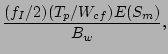
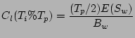
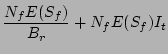
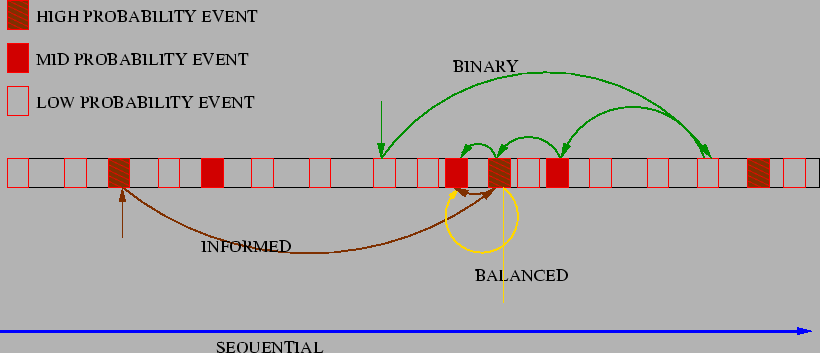
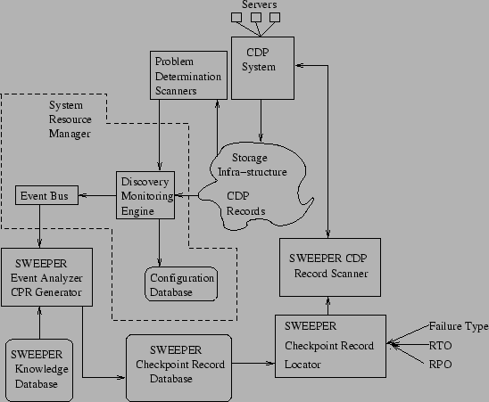
![\fbox{
\begin{minipage}[t]{0.6\textwidth}
\begin{tabular}{l}\small
{\em funct...
...end while}\\
{\em end locateCheckPoints}\\
\end{tabular}
\end{minipage}
}](SWEEPER_files/img59.png)
![% latex2html id marker 1119
\fbox{
\begin{minipage}[t]{0.65\textwidth}%
\begi...
...urrMin} \\
{\em end scanRecordsBalanced}\\
\end{tabular}
\end{minipage}
}](SWEEPER_files/img89.png)