|
||||||||||||||
|
Xiliang
Liu1, Kaliappa Ravindran2,
1
City University of
2
City College of
3
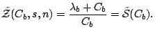
This paper analyzes the asymptotic behavior of packet-train
probing over a multi-hop network path ![]() carrying arbitrarily routed bursty cross-traffic flows.
We examine the statistical mean of the packet-train output dispersions and its
relationship to the input dispersion. We call this relationship the response
curve of path
carrying arbitrarily routed bursty cross-traffic flows.
We examine the statistical mean of the packet-train output dispersions and its
relationship to the input dispersion. We call this relationship the response
curve of path ![]() . We show that the real response curve
. We show that the real response curve ![]() is tightly lower-bounded by its multi-hop fluid
counterpart
is tightly lower-bounded by its multi-hop fluid
counterpart ![]() , obtained when every cross-traffic flow on
, obtained when every cross-traffic flow on ![]() is hypothetically replaced with a constant-rate fluid
flow of the same average intensity and routing pattern. The real curve
is hypothetically replaced with a constant-rate fluid
flow of the same average intensity and routing pattern. The real curve ![]() asymptotically approaches its fluid counterpart
asymptotically approaches its fluid counterpart ![]() as probing packet size or packet train length increases.
Most existing measurement techniques are based upon the single-hop fluid curve
as probing packet size or packet train length increases.
Most existing measurement techniques are based upon the single-hop fluid curve ![]() associated with the bottleneck link in
associated with the bottleneck link in ![]() . We note that the curve
. We note that the curve ![]() coincides with
coincides with ![]() in a certain large-dispersion input range, but falls
below
in a certain large-dispersion input range, but falls
below ![]() in the remaining small-dispersion input ranges. As an
implication of these findings, we show that bursty cross-traffic in multi-hop
paths causes negative bias (asymptotic underestimation) to most existing
techniques. This bias can be mitigated by reducing the deviation of
in the remaining small-dispersion input ranges. As an
implication of these findings, we show that bursty cross-traffic in multi-hop
paths causes negative bias (asymptotic underestimation) to most existing
techniques. This bias can be mitigated by reducing the deviation of ![]() from
from ![]() using large packet size or long packet-trains. However,
the bias is not completely removable for the techniques that use the portion of
using large packet size or long packet-trains. However,
the bias is not completely removable for the techniques that use the portion of
![]() that falls below
that falls below ![]() .
.
End-to-end estimation of the spare capacity along a network path using packet-train probing has recently become an important Internet measurement research area. Several measurement techniques such as TOPP [14], Pathload [6], IGI/PTR [5], Pathchirp [16], and Spruce [17] have been developed. Most of the current proposals use a single-hop path with constant-rate fluid cross-traffic to justify their methods. The behavior and performance of these techniques in a multi-hop path with general bursty cross-traffic is limited to experimental evaluations. Recent work [9] initiated the effort of developing an analytical foundation for bandwidth measurement techniques. Such a foundation is important in that it helps achieve a clear understanding of both the validity and the inadequacy of current techniques and provides a guideline to improve them. However, the analysis in [9] is restricted to single-hop paths. There is still a void to fill in understanding packet-train bandwidth estimation over a multi-hop network path.
Recall that the available bandwidth of a network hop is its residual
capacity after transmitting cross-traffic within a certain time interval. This
metric varies over time as well as a wide range of observation time intervals.
However, in this paper, we explicitly target the measurement of a long-term
average available bandwidth, which is a stable metric independent of
observation time instances and observation time intervals [9]. Consider an ![]() -hop
network path
-hop
network path ![]() , where the capacity of
link
, where the capacity of
link ![]() is denoted by
is denoted by ![]() and the long-term
average of the cross-traffic arrival rate at
and the long-term
average of the cross-traffic arrival rate at ![]() is given by
is given by ![]() , which is assumed to be less than
, which is assumed to be less than ![]() . The hop
available bandwidth of
. The hop
available bandwidth of ![]() is
is ![]() . The path available bandwidth
. The path available bandwidth ![]() is given by
is given by
The hop ![]() , which carries the minimum available
bandwidth, is called the tight link or the bottleneck linkIn general,
the tight link can be different from the link with the minimum capacity, which
we refer to as the narrow link of
, which carries the minimum available
bandwidth, is called the tight link or the bottleneck linkIn general,
the tight link can be different from the link with the minimum capacity, which
we refer to as the narrow link of ![]() .. That is,
.. That is,
The main idea of packet-train bandwidth estimation is to infer ![]() from the relationship between the
inter-packet dispersions of the output packet-trains and those of the input
packet-trains. Due to the complexity of this relationship in arbitrary network
paths with bursty cross-traffic flows, previous work simplifies the analysis
using a single-hop path with fluidWe use the term ``fluid" and
``constant-rate fluid" interchangeably. cross-traffic, while making the
following two assumptions without formal justification: first, cross-traffic
burstiness only causes measurement variability that can be smoothed out by
averaging multiple probing samples and second, non-bottleneck links have negligible
impact on the proposed techniques.
from the relationship between the
inter-packet dispersions of the output packet-trains and those of the input
packet-trains. Due to the complexity of this relationship in arbitrary network
paths with bursty cross-traffic flows, previous work simplifies the analysis
using a single-hop path with fluidWe use the term ``fluid" and
``constant-rate fluid" interchangeably. cross-traffic, while making the
following two assumptions without formal justification: first, cross-traffic
burstiness only causes measurement variability that can be smoothed out by
averaging multiple probing samples and second, non-bottleneck links have negligible
impact on the proposed techniques.
The validity of the first assumption is partially addressed in [9], where the authors use a single-hop path with bursty cross-traffic to derive the statistical mean of the packet-train output dispersions as a function of the input probing dispersion, referred to as the single-hop response curve. Their analysis shows that besides measurement variability, cross-traffic burstiness can also cause measurement bias to the techniques that are based on fluid analysis. This measurement bias cannot be reduced even when an infinite number of probing samples are used, but can be mitigated using long packet-trains and/or large probing packet size.
This paper addresses further the two assumptions that current techniques are based on. To this end, we extend the asymptotic analysis in [9] to arbitrary network paths and uncover the nature of the measurement bias caused by bursty cross-traffic flows in a multi-hop network path. This problem is significantly different from previous single-hop analysis due to the following reasons. First, unlike single-hop measurements, where the input packet-trains have deterministic and equal inter-packet separation formed by the probing source, the input packet-trains at any hop (except the first one) along a multi-link path are output from the previous hop and have random structure. Second and more importantly, the multi-hop probing asymptotics are strongly related to the routing pattern of cross-traffic flows. This issue never arises in a single-hop path and it has received little attention in prior investigation. However, as we show in this paper, it is one of the most significant factors that affect the accuracy of bandwidth measurement in multi-hop paths.
To characterize packet-train bandwidth estimation in its most general
settings, we derive the probing response curve ![]() of a multi-hop path
of a multi-hop path ![]() assuming arbitrarily routed bursty
cross-traffic flows. We compare
assuming arbitrarily routed bursty
cross-traffic flows. We compare ![]() with its multi-hop fluid counterpart
with its multi-hop fluid counterpart ![]() , which is a response curve obtained when
every cross-traffic flow in
, which is a response curve obtained when
every cross-traffic flow in ![]() is hypothetically replaced with a fluid flow
of the same average intensity and routing pattern. We show, under an ergodic
stationarity assumption for each cross-traffic flow, that the real curve
is hypothetically replaced with a fluid flow
of the same average intensity and routing pattern. We show, under an ergodic
stationarity assumption for each cross-traffic flow, that the real curve ![]() is tightly lower bounded by its fluid
counterpart
is tightly lower bounded by its fluid
counterpart ![]() and that the curve
and that the curve ![]() asymptotically approaches its fluid bound
asymptotically approaches its fluid bound ![]() in the entire input range as probing packet
size or packet-train length increases.
in the entire input range as probing packet
size or packet-train length increases.
Most of the existing techniques are based on the single-hop fluid response
curve ![]() associated with the bottleneck link in
associated with the bottleneck link in ![]() . Therefore, any deviation of the real curve
. Therefore, any deviation of the real curve ![]() from the single-hop curve
from the single-hop curve ![]() can potentially cause measurement bias in
bandwidth estimation. Note that the deviation
can potentially cause measurement bias in
bandwidth estimation. Note that the deviation ![]() can be decomposed as
can be decomposed as
The first term ![]() is always positive and causes
asymptotic underestimation of
is always positive and causes
asymptotic underestimation of ![]() for most of the existing techniques. This
deviation term and its resulting measurement bias are ``elastic" in the
sense that they can be reduced to a negligible level using packet-trains of
sufficient lengthThe analysis assumes infinite buffer space at each router..
For the second deviation term
for most of the existing techniques. This
deviation term and its resulting measurement bias are ``elastic" in the
sense that they can be reduced to a negligible level using packet-trains of
sufficient lengthThe analysis assumes infinite buffer space at each router..
For the second deviation term ![]() , we note that both
, we note that both ![]() and
and ![]() are piece-wise linear curves. The first two
linear segments in
are piece-wise linear curves. The first two
linear segments in ![]() associated with large input dispersions
coincide with
associated with large input dispersions
coincide with ![]() (i.e.,
(i.e., ![]() ). The rest of the linear
segments in
). The rest of the linear
segments in ![]() associated with small input dispersions
appear above
associated with small input dispersions
appear above ![]() (i.e.,
(i.e., ![]() ). The amount of deviation
and the additional negative measurement bias it causes are dependent on the
routing patterns of cross-traffic flows, and are maximized when every flow
traverses only one hop along the path (which is often called one-hop
persistent cross-traffic routing [4]).
Furthermore, the curve deviation
). The amount of deviation
and the additional negative measurement bias it causes are dependent on the
routing patterns of cross-traffic flows, and are maximized when every flow
traverses only one hop along the path (which is often called one-hop
persistent cross-traffic routing [4]).
Furthermore, the curve deviation ![]() is ``non-elastic" and stays
constant with respect to probing packet size and packet-train length at any
given input rate. Therefore, the measurement bias it causes cannot be overcome
by adjusting the input packet-train parameters.
is ``non-elastic" and stays
constant with respect to probing packet size and packet-train length at any
given input rate. Therefore, the measurement bias it causes cannot be overcome
by adjusting the input packet-train parameters.
Among current measurement techniques, pathload and PTR operate in the input
probing range where ![]() coincides with
coincides with ![]() , and consequently are only subject to the
measurement bias caused by the first deviation term
, and consequently are only subject to the
measurement bias caused by the first deviation term ![]() . Spruce may use the probing
range where
. Spruce may use the probing
range where ![]() . Hence it is subject to
both elastic and non-elastic negative measurement biases. The amount of bias
can be substantially more than the actual available bandwidth in certain common
scenarios, leading to negative results by the measurement algorithm and a final
estimate of zero by the tool.
. Hence it is subject to
both elastic and non-elastic negative measurement biases. The amount of bias
can be substantially more than the actual available bandwidth in certain common
scenarios, leading to negative results by the measurement algorithm and a final
estimate of zero by the tool.
The rest of the paper is organized as follows. Section 2
derives the multi-hop response curve ![]() assuming arbitrarily routed fluid
cross-traffic flows and examines the deviation term
assuming arbitrarily routed fluid
cross-traffic flows and examines the deviation term ![]() . In Section 3
and 4, we derive the real response curve
. In Section 3
and 4, we derive the real response curve ![]() of a multi-hop path and show its relationship
to its fluid counterpart
of a multi-hop path and show its relationship
to its fluid counterpart ![]() . We provide practical evidence for our
theoretical results using testbed experiments and real Internet measurements in
Section 5. We examine the impact of these results on
existing techniques in Section 6 and summarize related work
in Section 7. Finally, we briefly discuss future work and
conclude in Section 8.
. We provide practical evidence for our
theoretical results using testbed experiments and real Internet measurements in
Section 5. We examine the impact of these results on
existing techniques in Section 6 and summarize related work
in Section 7. Finally, we briefly discuss future work and
conclude in Section 8.
Due to limited space, most of the proofs in this paper are omitted, and we refer interested readers to [10] for more technical details.
It is important to first thoroughly understand the response
curve ![]() of a network path carrying fluid
cross-traffic flows, since as we show later, the fluid curve
of a network path carrying fluid
cross-traffic flows, since as we show later, the fluid curve ![]() is an approachable bound of the real
response curve
is an approachable bound of the real
response curve ![]() . Initial investigation of the fluid curves
is due to Melandar et al. [13]
and Dovrolis et al. [3].
However, prior work only considers two special cross-traffic routing cases
(one-hop persistent routing and path persistent routing). In this section, we
formulate and solve the problem for arbitrary cross-traffic routing patterns,
based on which, we discuss several important properties of the fluid response
curves that allow us to obtain the path available bandwidth information.
. Initial investigation of the fluid curves
is due to Melandar et al. [13]
and Dovrolis et al. [3].
However, prior work only considers two special cross-traffic routing cases
(one-hop persistent routing and path persistent routing). In this section, we
formulate and solve the problem for arbitrary cross-traffic routing patterns,
based on which, we discuss several important properties of the fluid response
curves that allow us to obtain the path available bandwidth information.
We first introduce necessary notations to formulate a multi-hop path and the cross-traffic flows that traverse along the path.
An ![]() -hop network path
-hop network path ![]() is a sequence of
is a sequence of ![]() interconnected First-Come First-Served (FCFS) store-and-forward
hops. For each forwarding hop
interconnected First-Come First-Served (FCFS) store-and-forward
hops. For each forwarding hop ![]() in
in ![]() , we denote its link capacity by
, we denote its link capacity by ![]() , and assume that it has infinite buffer space and a
work-conserving queuing discipline. Suppose that there are
, and assume that it has infinite buffer space and a
work-conserving queuing discipline. Suppose that there are ![]() fluid
cross-traffic flows traversing path
fluid
cross-traffic flows traversing path ![]() . The rate of flow
. The rate of flow ![]() is denoted by
is denoted by
![]() and the flow rate vector is given by
and the flow rate vector is given by ![]() .
.
We impose two routing constraints on cross-traffic flows to simplify the discussion. The first constraint requires every flow to have a different routing pattern. In the case of otherwise, the flows with the same routing pattern should be aggregated into one single flow. The second routing constraint requires every flow to have only one link where it enters the path and also have only one (downstream) link where it exits from the path. In the case of otherwise, the flow is decomposed into several separate flows that meet this routing constraint.
Definition 1 A flow aggregation is a set of
flows, represented by a ``selection vector" ![]() , where
, where ![]() if flow
if flow ![]() belongs to the aggregation and
belongs to the aggregation and ![]() if otherwise. We use
if otherwise. We use ![]() to represent the selection vector of the
aggregation that contains flow
to represent the selection vector of the
aggregation that contains flow ![]() alone.
alone.
There are several operations between flow aggregations. First, the common
flows to aggregations ![]() and
and ![]() form another aggregation, whose selection
vector is given by
form another aggregation, whose selection
vector is given by ![]() , where the operator
, where the operator ![]() represents ``element-wise multiplication." Second, the
aggregation that contains the flows in
represents ``element-wise multiplication." Second, the
aggregation that contains the flows in ![]() but not in
but not in ![]() is given by
is given by ![]() . Finally, note that
the traffic intensity of aggregation
. Finally, note that
the traffic intensity of aggregation ![]() can be computed from the inner product
can be computed from the inner product ![]() .
.
We now define several types of flow aggregation frequently used in this
paper. First, the traversing flow aggregation at link ![]() , denoted
by its selection vector
, denoted
by its selection vector ![]() , includes all fluid flows that pass through
, includes all fluid flows that pass through
![]() . The
. The ![]() matrix
matrix ![]() becomes the routing matrix of path
becomes the routing matrix of path ![]() . For convenience, we define an auxiliary
selection vector
. For convenience, we define an auxiliary
selection vector ![]() .
.
The second type of flow aggregation, denoted by ![]() , includes all flows entering the path at
link
, includes all flows entering the path at
link ![]() , which can be expressed as
, which can be expressed as ![]() given the second routing constraint stated previously. The third
type of flow aggregation, which includes flows that enter the path at link
given the second routing constraint stated previously. The third
type of flow aggregation, which includes flows that enter the path at link ![]() and traverse the downstream link
and traverse the downstream link ![]() , is denoted as
, is denoted as ![]() , where
, where ![]() .
.
The cross-traffic intensity at link ![]() is denoted by
is denoted by ![]() . We assume
. We assume ![]() for
for ![]() . Since none of the links in
. Since none of the links in ![]() is congested, the arrival rate of flow
is congested, the arrival rate of flow ![]() at any link it traverses is
at any link it traverses is ![]() . Consequently, we
have
. Consequently, we
have
We further define the path configuration of ![]() as the following
as the following ![]() matrix
matrix
The hop available bandwidth of ![]() is given by
is given by ![]() . We assume that every hop has
different available bandwidth, and consequently that the tight link is unique.
Sometimes, we also need to refer to the second minimum hop available bandwidth
and the associated link, which we denote as
. We assume that every hop has
different available bandwidth, and consequently that the tight link is unique.
Sometimes, we also need to refer to the second minimum hop available bandwidth
and the associated link, which we denote as ![]() and
and ![]() ,
respectively. That is
,
respectively. That is
where ![]() is the index of the tight hop.
is the index of the tight hop.
We now consider a packet-train of input dispersion (i.e., inter-packet
spacing) ![]() and packet size
and packet size ![]() that is used to probe
path
that is used to probe
path ![]() . We are interested in computing the output
dispersion of the packet train and examining its relation to
. We are interested in computing the output
dispersion of the packet train and examining its relation to ![]() .
Such a relation is called the gap response curve of path
.
Such a relation is called the gap response curve of path ![]() . It is easy to verify that under fluid
conditions, the response curve does not depend on the packet-train length
. It is easy to verify that under fluid
conditions, the response curve does not depend on the packet-train length ![]() . Hence, we only consider the case of packet-pair probing. We
denote the output dispersion at link
. Hence, we only consider the case of packet-pair probing. We
denote the output dispersion at link ![]() as
as ![]() or
or ![]() for short, and
again for notational convenience we let
for short, and
again for notational convenience we let ![]() . Note that
. Note that ![]() corresponds to the notation
corresponds to the notation ![]() we have used previously.
we have used previously.
Based on our formulations, the gap response curve of path ![]() has a recursive representation given below.
has a recursive representation given below.
Theorem 1 When a
packet-pair with input dispersion ![]() and packet size
and packet size ![]() is used to probe an
is used to probe an ![]() -hop fluid path with
routing matrix
-hop fluid path with
routing matrix ![]() and flow rate vector
and flow rate vector ![]() , the output dispersion at link
, the output dispersion at link ![]() can
be recursively expressed as
can
be recursively expressed as
where ![]() is The term
is The term ![]() represents the volume of fluid cross-traffic buffered between the
packet-pair in the outgoing queue of link
represents the volume of fluid cross-traffic buffered between the
packet-pair in the outgoing queue of link ![]() . For an analogical
understanding, we can view the packet-pair as a bus, the cross-traffic as
passengers, and the routers as bus stations. Then,
. For an analogical
understanding, we can view the packet-pair as a bus, the cross-traffic as
passengers, and the routers as bus stations. Then, ![]() is the
amount of cross-traffic picked up by the packet-pair at link
is the
amount of cross-traffic picked up by the packet-pair at link ![]() as
well as all the upstream links of
as
well as all the upstream links of ![]() . This cross-traffic
will traverse over link
. This cross-traffic
will traverse over link ![]() due to the flows' routing decision.
due to the flows' routing decision.
Proof. Assumes that the first probing packet arrives
at link ![]() at time instance
at time instance ![]() . It gets immediate
transmission service and departs at
. It gets immediate
transmission service and departs at ![]() . The second
packet arrives at
. The second
packet arrives at ![]() . The server of
. The server of ![]() needs to
transmit
needs to
transmit ![]() amount of data before it can serve the second
packet. If this is done before time instance
amount of data before it can serve the second
packet. If this is done before time instance ![]() , the second packet also gets immediate
service and
, the second packet also gets immediate
service and ![]() . Otherwise, the sever undergoes a
busy period between the departure of the two packets, meaning that
. Otherwise, the sever undergoes a
busy period between the departure of the two packets, meaning that ![]() . Therefore, we have
. Therefore, we have
|
|
(9) |
This completes the proof of the theorem. ![]()
As a quick sanity check, we verify the compatibility between Theorem 1 and the special one-hop persistent routing case, where
every flow that enters the path at link ![]() will exit the path at
link
will exit the path at
link ![]() . For this routing pattern, we have
. For this routing pattern, we have
|
|
(10) |
Therefore, equation (8) can be
simplified as
which agrees with previous results [3], [13].
Theorem 1 leads to several important properties of the
fluid response curve ![]() , which we discuss next. These properties
tell us how bandwidth information can be extracted from the curve
, which we discuss next. These properties
tell us how bandwidth information can be extracted from the curve ![]() , and also show the deviation of
, and also show the deviation of ![]() , as one should be aware of, from the
single-hop fluid curve
, as one should be aware of, from the
single-hop fluid curve ![]() of the tight link.
of the tight link.
Property 1 The output
dispersion ![]() is a continuous piece-wise linear
function of the input dispersion
is a continuous piece-wise linear
function of the input dispersion ![]() in the input
dispersion range
in the input
dispersion range ![]() .
.
Let ![]() be the input dispersion turning points that split the gap response
curve to
be the input dispersion turning points that split the gap response
curve to ![]() linear segmentsNote that the turning points in
linear segmentsNote that the turning points in ![]() is indexed according to the decreasing order
of their values. The reason will be clear shortly when we discuss the rate
response curve.. Our next result discusses the turning points and linear
segments that are of major importance in bandwidth estimation.
is indexed according to the decreasing order
of their values. The reason will be clear shortly when we discuss the rate
response curve.. Our next result discusses the turning points and linear
segments that are of major importance in bandwidth estimation.
Property 2 The first
turning point ![]() corresponds to the path available bandwidth in
the sense that
corresponds to the path available bandwidth in
the sense that ![]() . The first linear segment in
the input dispersion range
. The first linear segment in
the input dispersion range ![]() has slope 1 and
intercept 0. The second linear segment in the input dispersion range
has slope 1 and
intercept 0. The second linear segment in the input dispersion range ![]() has slope
has slope ![]() and intercept
and intercept ![]() , where
, where ![]() is the index of the tight link:
is the index of the tight link:
These facts are irrespective of the routing matrix.
It helps to find the expression for the turning point ![]() , so that we can identify the exact range for the second linear
segment. However, unlike
, so that we can identify the exact range for the second linear
segment. However, unlike ![]() , the turning point
, the turning point ![]() is dependent on the routing matrix. In fact, all other turning
points are dependent on the routing matrix and can not be computed based on the
path configuration matrix alone. Therefore, we only provide a bound for
is dependent on the routing matrix. In fact, all other turning
points are dependent on the routing matrix and can not be computed based on the
path configuration matrix alone. Therefore, we only provide a bound for ![]() .
.
Property 3 For any
routing matrix, the term ![]() is no less than
is no less than ![]() , which
is the second minimum hop available bandwidth of path
, which
is the second minimum hop available bandwidth of path ![]() .
.
The slopes and intercepts for all but the first two linear segments are related to the routing matrix. We skip the derivation of their expressions, but instead provide both a lower bound and an upper bound for the entire response curve.
Property 4 For a
given path configuration matrix, the gap response curve associated with any
routing matrix is lower bounded by the single-hop gap response curve of the
tight link
It is upper bounded by the gap response curve associated with one-hop persistent routing.
We now make several observations regarding the deviation of ![]() (i.e.,
(i.e., ![]() ) from
) from ![]() . Combing (12) and
(13), we see that
. Combing (12) and
(13), we see that ![]() when
when ![]() . That is, the first two linear segments
on
. That is, the first two linear segments
on ![]() coincide with
coincide with ![]() . When
. When ![]() , Property 4
implies that the deviation
, Property 4
implies that the deviation ![]() is positive. The exact
value depends on cross-traffic routing and it is maximized in one-hop
persistent routing for any given path configuration matrix.
is positive. The exact
value depends on cross-traffic routing and it is maximized in one-hop
persistent routing for any given path configuration matrix.
Also note that there are three pieces of path information that we can
extract from the gap response curve ![]() without knowing the routing matrix. By
locating the first turning point
without knowing the routing matrix. By
locating the first turning point ![]() , we can compute
the path available bandwidth. From the second linear segment, we can obtain the
tight link capacity and cross-traffic intensity (and consequently, the
bottleneck link utilization) information. Other parts of the response curve
, we can compute
the path available bandwidth. From the second linear segment, we can obtain the
tight link capacity and cross-traffic intensity (and consequently, the
bottleneck link utilization) information. Other parts of the response curve ![]() are less readily usable due to their
dependence on cross-traffic routing.
are less readily usable due to their
dependence on cross-traffic routing.
To extract bandwidth information from the output dispersion ![]() , it is often more helpful to look at the rate response
curve, i.e., the functional relation between the output rate
, it is often more helpful to look at the rate response
curve, i.e., the functional relation between the output rate ![]() and the input rate
and the input rate ![]() .
However, since this relation is not linear, we adopt a transformed version
first proposed by Melander et al. [14], which depicts the relation
between the ratio
.
However, since this relation is not linear, we adopt a transformed version
first proposed by Melander et al. [14], which depicts the relation
between the ratio ![]() and
and ![]() . Denoting
this rate response curve by
. Denoting
this rate response curve by ![]() , we have
, we have
This transformed version of the rate response curve is also piece-wise
linear. It is easy to see that the first turning point in the rate curve is ![]() and that the rate curve in the input rate
range
and that the rate curve in the input rate
range ![]() can be expressed as
can be expressed as
Finally, it is also important to notice that the rate response curve ![]() does not depend on the probing
packet size
does not depend on the probing
packet size ![]() . This is because, for any given input rate
. This is because, for any given input rate ![]() , both
, both ![]() and
and ![]() are proportional to
are proportional to ![]() . Consequently, the ratio between these two terms remains a
constant for any
. Consequently, the ratio between these two terms remains a
constant for any ![]() .
.
We use a simple example to illustrate the properties of the
fluid response curves. Suppose that we have a 3-hop path with equal capacity ![]() mb/s,
mb/s, ![]() . We consider two routing matrices
and flow rate settings that lead to the same link load at each hop.
. We consider two routing matrices
and flow rate settings that lead to the same link load at each hop.
In the first setting, the flow rate vector ![]() and the routing pattern is one-hop
persistent, i.e.,
and the routing pattern is one-hop
persistent, i.e., ![]() diag
diag![]() . In the second
setting, the flow rate vector
. In the second
setting, the flow rate vector ![]() and the routing pattern is path
persistent. That is,
and the routing pattern is path
persistent. That is,
Both of the settings result in the same path configuration
matrix
The probing packet size ![]() is
is ![]() bytes. The fluid
gap response curves for the two routing patterns are plotted in Fig. 1(a). In this example, both curves have 4 linear segments
separated by turning points
bytes. The fluid
gap response curves for the two routing patterns are plotted in Fig. 1(a). In this example, both curves have 4 linear segments
separated by turning points ![]() ms,
ms, ![]() ms, and
ms, and ![]() ms. Note that part of the curve for
path-persistent routing appears below the one for one-hop persistent routing.
The lower bound
ms. Note that part of the curve for
path-persistent routing appears below the one for one-hop persistent routing.
The lower bound ![]() identified in Property 4
is also plotted in the figure. This lower bound is the gap response curve of
the single-hop path comprising only the tight link
identified in Property 4
is also plotted in the figure. This lower bound is the gap response curve of
the single-hop path comprising only the tight link ![]() .
.
The rate response curves for the two examples are given in Fig. 1(b), where the three turning points are ![]() mb/s,
mb/s,
![]() mb/s, and
mb/s, and ![]() mb/s respectively. Due to the
transformation we adopted, the rate curve for one-hop persistent routing still
remains as an upper bound for the rate curves associated with the other routing
patterns. From Fig. 1(b), we also see that, similar to
the gap curves, the two multi-hop rate response curves and their lower bound
mb/s respectively. Due to the
transformation we adopted, the rate curve for one-hop persistent routing still
remains as an upper bound for the rate curves associated with the other routing
patterns. From Fig. 1(b), we also see that, similar to
the gap curves, the two multi-hop rate response curves and their lower bound ![]() (i.e., the transformed rate
version of
(i.e., the transformed rate
version of ![]() ) share the same first and second
linear segments.
) share the same first and second
linear segments.
We conclude this section by discussing several major
challenges in extending the response curve analysis to a multi-hop path
carrying bursty cross-traffic flows. First, notice that with bursty cross-traffic,
even when the input dispersion and packet-train parameters remain constant, the
output dispersion becomes random, rather than deterministic as in fluid
cross-traffic. The gap response curve ![]() , defined as the functional relation between
the statistical mean of the output dispersion and the input dispersion, is much
more difficult to penetrate than the fluid curve
, defined as the functional relation between
the statistical mean of the output dispersion and the input dispersion, is much
more difficult to penetrate than the fluid curve ![]() . Second, unlike in the fluid case, where
both packet-train length
. Second, unlike in the fluid case, where
both packet-train length ![]() and probing packet size
and probing packet size ![]() have
no impact on the rate response curve
have
no impact on the rate response curve ![]() , the response curves in bursty
cross-traffic are strongly related to these two packet-train parameters.
Finally, a full characterization of a fluid flow only requires one parameter -
its arrival rate, while a full characterization of a bursty flow requires
several stochastic processes. In what follows, we address these problems and extend
our analysis to multi-hop paths with bursty cross-traffic.
, the response curves in bursty
cross-traffic are strongly related to these two packet-train parameters.
Finally, a full characterization of a fluid flow only requires one parameter -
its arrival rate, while a full characterization of a bursty flow requires
several stochastic processes. In what follows, we address these problems and extend
our analysis to multi-hop paths with bursty cross-traffic.
In this section, we present a stochastic formulation of the multi-hop bandwidth measurement problem and derive a recursive expression for the output dispersion random variable. This expression is a fundamental result that the asymptotic analysis in Section 4 is based upon.
We keep most of the notations the same as in the previous section, although some of the terms are extended to have a different meaning, which we explain shortly. Since cross-traffic flows now become bursty flows of data packets, we adopt the definitions of several random processes (Definition 1-6) in [9] to characterize them. However, these definitions need to be refined to be specific to a given router and flow aggregation. In what follows, we only give the definitions of two random processes and skip the others. The notations for all six random processes are given in Table 3.1.
Definition 2 The cumulative traffic arrival
process of flow aggregation ![]() at link
at link ![]() , denoted as
, denoted as ![]() is a
random process counting the total amount of data (in bits) received by hop
is a
random process counting the total amount of data (in bits) received by hop ![]() from flow aggregation
from flow aggregation ![]() up to time instance
up to time instance ![]() .
.
Definition 3 Hop workload process of ![]() with respect to flow aggregation
with respect to flow aggregation ![]() , denoted as
, denoted as ![]() indicates the
sum at time instance
indicates the
sum at time instance ![]() of service times of all packets in the
queue and the remaining service time of the packet in service, assuming that
flow aggregation
of service times of all packets in the
queue and the remaining service time of the packet in service, assuming that
flow aggregation ![]() is the only traffic passing through link
is the only traffic passing through link ![]() .
.
We next make several modeling assumptions on cross-traffic flows. First, we assume that all flows have stationary arrivals.
Assumption 1 For any
cross-traffic flow ![]() that enters the path from link
that enters the path from link ![]() , the cumulative traffic arrival process
, the cumulative traffic arrival process ![]() has ergodic stationary
increments. That is, for any
has ergodic stationary
increments. That is, for any ![]() , the
, the ![]() -interval
traffic intensity process
-interval
traffic intensity process ![]() is a mean-square ergodic
process with time-invariant distribution and ensemble mean
is a mean-square ergodic
process with time-invariant distribution and ensemble mean ![]() .
.
We explain this assumption in more details. First, the stationary increment
assumption implies that the increment process of ![]() for any given time interval
for any given time interval ![]() , namely
, namely ![]() , has a time-invariant distribution. This further implies that the
, has a time-invariant distribution. This further implies that the
![]() -interval traffic intensity process
-interval traffic intensity process ![]() is identically
distributed, whose marginal distribution at any time instance
is identically
distributed, whose marginal distribution at any time instance ![]() can be described by the same random variable
can be described by the same random variable ![]() . Second, the mean-square
ergodicity implies that, as the observation interval
. Second, the mean-square
ergodicity implies that, as the observation interval ![]() increases,
the random variable
increases,
the random variable ![]() converges to
converges to ![]() in
the mean-square sense. In other words, the variance of
in
the mean-square sense. In other words, the variance of ![]() decays to 0 as
decays to 0 as ![]() , i.e.,
, i.e.,
Our next assumption states the independent relationship between different
flows that enter path ![]() at the same link.
at the same link.
Assumption 2 For any
two flows ![]() and
and ![]() that enter the path at link
that enter the path at link ![]() , the two processes
, the two processes ![]() and
and ![]() are independent. Specifically,
for any two time instances
are independent. Specifically,
for any two time instances ![]() and
and ![]() , the two random variables
, the two random variables
![]() and
and ![]() are independent.
are independent.
As a consequence of the two assumptions we made, the ergodic stationary property also holds for any flow aggregations at their entering link.
|
Corollary 1 For any
flow aggregation ![]() that enters the path at link
that enters the path at link ![]() ,
i.e.,
,
i.e., ![]() , the process
, the process ![]() has ergodic stationary increments.
Consequently, the traffic intensity random variable
has ergodic stationary increments.
Consequently, the traffic intensity random variable ![]() converges to
converges to ![]() in the mean-square sense
in the mean-square sense
Due to Szczotka [18], [19], the workload process ![]() will ``inherit" the ergodic
stationarity property from the traffic arrival process
will ``inherit" the ergodic
stationarity property from the traffic arrival process ![]() . This property is further carried
over to the
. This property is further carried
over to the ![]() -interval workload-difference process
-interval workload-difference process ![]() and the available
bandwidth process
and the available
bandwidth process ![]() . This distributional
stationarity allows us to focus on the corresponding random variables
. This distributional
stationarity allows us to focus on the corresponding random variables ![]() ,
, ![]() , and
, and ![]() . It is easy to get, from their
definitions, that the statistical means of
. It is easy to get, from their
definitions, that the statistical means of ![]() and
and ![]() are 0 and
are 0 and ![]() , respectivelyNote that the hop available
bandwidth of link
, respectivelyNote that the hop available
bandwidth of link ![]() that is of measurement interest, given
by
that is of measurement interest, given
by ![]() can be less than
can be less than ![]() .. Further, the ergodicity property leads
to the following result.
.. Further, the ergodicity property leads
to the following result.
Lemma 1 For any flow
aggregation ![]() that enter the path at link
that enter the path at link ![]() ,
the random variable
,
the random variable ![]() converges in the mean-square
sense to
converges in the mean-square
sense to ![]() as
as ![]() , i.e.,
, i.e.,
On the other hand, notice that unlike ![]() and
and ![]() , the workload-difference
process
, the workload-difference
process ![]() is not a moving average
process by nature. Consequently, the mean-square ergodicity of
is not a moving average
process by nature. Consequently, the mean-square ergodicity of ![]() does not cause the
variance of
does not cause the
variance of ![]() to decay with respect to the
increase of
to decay with respect to the
increase of ![]() . Instead, we have the following lemma.
. Instead, we have the following lemma.
To obtain our later results, not only do we need to know the asymptotic
variance of ![]() ,
, ![]() and
and ![]() when
when ![]() approaches
infinity, but also we often rely on their variance being uniformly bounded (for
any
approaches
infinity, but also we often rely on their variance being uniformly bounded (for
any ![]() ) by some constant. This condition can be easily
justified from a practical standpoint. First note that cross-traffic arrival
rate is bounded by the capacities of incoming links at a given router. Suppose
that the sum of all incoming link capacities at hop
) by some constant. This condition can be easily
justified from a practical standpoint. First note that cross-traffic arrival
rate is bounded by the capacities of incoming links at a given router. Suppose
that the sum of all incoming link capacities at hop ![]() is
is ![]() , then
, then ![]() is distributed in a finite
interval
is distributed in a finite
interval ![]() and its variance is uniformly bounded by the
constant
and its variance is uniformly bounded by the
constant ![]() for any observation interval
for any observation interval ![]() . Similarly, the variance of
. Similarly, the variance of ![]() is uniformly bounded by the
constant
is uniformly bounded by the
constant ![]() . The variance of
. The variance of ![]() is uniformly bounded by the
constant
is uniformly bounded by the
constant ![]() for any
for any ![]() , which
directly follows from the definition of
, which
directly follows from the definition of ![]() .
.
Finally, we remind that some of the notations introduced in Section 2.1 now
are used with a different meaning. The rate of the bursty cross-traffic flow ![]() , denoted by
, denoted by ![]() , is the probabilistic mean of the
traffic intensity random variable
, is the probabilistic mean of the
traffic intensity random variable ![]() , which is also the long-term
average arrival rate of flow
, which is also the long-term
average arrival rate of flow ![]() at any link it
traverses. The term
at any link it
traverses. The term ![]() becomes the long-term
average arrival rate of the aggregated cross-traffic at link
becomes the long-term
average arrival rate of the aggregated cross-traffic at link ![]() .
The term
.
The term ![]() is the long-term average hop available
bandwidth at link
is the long-term average hop available
bandwidth at link ![]() . Again recall that we explicitly
target the measurement of long-term averages of available bandwidth and/or
cross-traffic intensity, instead of the corresponding metrics in a certain time
interval.
. Again recall that we explicitly
target the measurement of long-term averages of available bandwidth and/or
cross-traffic intensity, instead of the corresponding metrics in a certain time
interval.
We now consider an infinite series of packet-trains with
input inter-packet dispersion ![]() , packet size
, packet size ![]() , and
packet-train length
, and
packet-train length ![]() . This series is driven to path
. This series is driven to path ![]() by a point process
by a point process ![]() with sufficient
large inter-probing separation. Let
with sufficient
large inter-probing separation. Let ![]() and
and ![]() be the departure time instances from link
be the departure time instances from link ![]() of the
first and last probing packets in the
of the
first and last probing packets in the ![]() packet-train. We
define the sampling interval of the packet-train as the total spacing
packet-train. We
define the sampling interval of the packet-train as the total spacing ![]() , and the output dispersion
as the average spacing
, and the output dispersion
as the average spacing ![]() of the packet-train. Both
of the packet-train. Both ![]() and
and ![]() are random variables, whose statistics might
depend on several factors such as the input dispersion
are random variables, whose statistics might
depend on several factors such as the input dispersion ![]() , the
packet-train parameters
, the
packet-train parameters ![]() and
and ![]() , the packet-train
index
, the packet-train
index ![]() in the probing series, and the hop
in the probing series, and the hop ![]() that
the output dispersion
that
the output dispersion ![]() is associated with. Therefore, a full
version of
is associated with. Therefore, a full
version of ![]() is written as
is written as ![]() . However, for notation brevity, we
often omit the parameters that have little relevance to the topic under
discussion.
. However, for notation brevity, we
often omit the parameters that have little relevance to the topic under
discussion.
We now formally state the questions we address in this paper. Note that a
realization of the stochastic process ![]() is just a
packet-train probing experiment. We examine the sample-path time-average of
this process and its relationship to
is just a
packet-train probing experiment. We examine the sample-path time-average of
this process and its relationship to ![]() when keeping
when keeping ![]() and
and ![]() constant. This relationship, previously
denoted by
constant. This relationship, previously
denoted by ![]() , is called the gap response curve of path
, is called the gap response curve of path ![]() .
.
Notice that the ergodic stationarity of cross-traffic arrival, as we assumed
previously, can reduce our response curve analysis to the investigation of a
single random variable. This is because each packet-train comes to see a
multi-hop system of the same stochastic nature and the output dispersion
process ![]() is an identically
distributed random sequence, which can be described by the output
dispersion random variable
is an identically
distributed random sequence, which can be described by the output
dispersion random variable ![]() . The sample-path time average of the
output dispersion process coincides with the mean of the random variable
. The sample-path time average of the
output dispersion process coincides with the mean of the random variable ![]() Note that the output dispersion process can be correlated.
However, this does not affect the sample-path time average of the process..
Therefore, in the rest of the paper, we focus on the statistics of
Note that the output dispersion process can be correlated.
However, this does not affect the sample-path time average of the process..
Therefore, in the rest of the paper, we focus on the statistics of ![]() and drop the index
and drop the index ![]() .
.
In our later analysis, we compare the gap response curve of ![]() with that of the fluid counterpart of
with that of the fluid counterpart of ![]() and prove that the former is lower-bounded by
the latter.
and prove that the former is lower-bounded by
the latter.
Definition 4 Suppose
that path ![]() has a routing matrix
has a routing matrix ![]() and a flow rate vector
and a flow rate vector ![]() and that path
and that path ![]() has a routing matrix
has a routing matrix ![]() and a flow rate vector
and a flow rate vector ![]() .
. ![]() is called the fluid counterpart of
is called the fluid counterpart of ![]() if 1) all cross-traffic flows traversing
if 1) all cross-traffic flows traversing ![]() are constant-rate fluid; 2) the two
paths
are constant-rate fluid; 2) the two
paths ![]() and
and ![]() have the same configuration matrix; and 3)
there exists a row-exchange matrix
have the same configuration matrix; and 3)
there exists a row-exchange matrix ![]() , such that
, such that ![]() and
and ![]() .
.
From this definition, we see that for every flow ![]() in
in ![]() , there is a corresponding fluid flow
, there is a corresponding fluid flow ![]() in the fluid counterpart of
in the fluid counterpart of ![]() such that flow
such that flow ![]() have the
same average intensity and routing pattern as those of flow
have the
same average intensity and routing pattern as those of flow ![]() .
Note that the third condition in Definition 4 is
made to allow the two flows have different indices, i.e., to allow
.
Note that the third condition in Definition 4 is
made to allow the two flows have different indices, i.e., to allow ![]() .
.
A second focus of this paper is to study the impact of packet-train
parameters ![]() and
and ![]() on the response curves. That is, for any
given input rate
on the response curves. That is, for any
given input rate ![]() and other parameters fixed, we examine
the convergence properties of the output dispersion random variable
and other parameters fixed, we examine
the convergence properties of the output dispersion random variable ![]() as
as ![]() or
or ![]() tends
to infinity.
tends
to infinity.
We keep input packet-train parameters ![]() ,
, ![]() ,
and
,
and ![]() constant and next obtain a basic expression for the output
dispersion random variable
constant and next obtain a basic expression for the output
dispersion random variable ![]() .
.
Lemma 3 Letting ![]() , the random variable
, the random variable ![]() has the following
recursive expression
has the following
recursive expression
where the term ![]() is a random variable representing the
extra queuing delaySee section 3.2 in [9]
for more discussions about this term in a single-hop context, where
is a random variable representing the
extra queuing delaySee section 3.2 in [9]
for more discussions about this term in a single-hop context, where ![]() is referred to as intrusion residual. (besides the queuing delay
caused by the workload process
is referred to as intrusion residual. (besides the queuing delay
caused by the workload process ![]() ) experienced at
) experienced at ![]() by
the last probing packet in the train. The term
by
the last probing packet in the train. The term ![]() is another random variable indicating the hop
idle time of
is another random variable indicating the hop
idle time of ![]() during the sampling interval of the packet train.
during the sampling interval of the packet train.
This result is very similar to Lemma 5 in [9]. However, due to the random input
packet-train structure at ![]() , all but the term
, all but the term ![]() in (22) become random variables. Some terms,
such as
in (22) become random variables. Some terms,
such as ![]() and
and ![]() , even have two
dimensions of randomness. To understand the behavior of probing response
curves, we need to investigate the statistical properties of each term in (22).
, even have two
dimensions of randomness. To understand the behavior of probing response
curves, we need to investigate the statistical properties of each term in (22).
In this section, we first show that the gap response curve ![]() of a multi-hop path
of a multi-hop path ![]() is lower bounded by its fluid counterpart
is lower bounded by its fluid counterpart ![]() . We then investigate the
impact of packet-train parameters on
. We then investigate the
impact of packet-train parameters on ![]() .
.
Our next lemma shows that passing through a link can only increase the dispersion random variable in mean.
Lemma 4 For ![]() , the output dispersion random variable
, the output dispersion random variable ![]() has a mean no less than that of
has a mean no less than that of ![]() . That is,
. That is, ![]() .
.
Using the first part of (22), our next lemma shows that
for any link ![]() , the output dispersion random variable
, the output dispersion random variable ![]() is lower bounded in mean by a linear combination of the output
dispersion random variables
is lower bounded in mean by a linear combination of the output
dispersion random variables ![]() , where
, where ![]() .
.
From Lemma 4 and Lemma 5, we
get
This leads to the following theorem.
Theorem 2 For any
input dispersion ![]() , packet-train parameters
, packet-train parameters ![]() and
and ![]() , the output dispersion random variable
, the output dispersion random variable ![]() of path
of path ![]() is lower bounded in mean by the output
dispersion
is lower bounded in mean by the output
dispersion ![]() of the fluid counterpart of
of the fluid counterpart of ![]() :
:
Proof. We apply mathematical induction to ![]() . When
. When ![]() ,
, ![]() . Assuming that (25)
holds for
. Assuming that (25)
holds for ![]() , we next prove that it also holds for
, we next prove that it also holds for ![]() . Recalling (24), we have
. Recalling (24), we have
|
|
|
|
|
|
|
|
|
|
where the second inequality is due to the induction hypothesis, and the last
equality is because of Theorem 1. ![]()
Theorem 2 shows that in the entire input gap range,
the piece-wise linear fluid gap response curve ![]() discussed in Section 2 is
a lower bound of the real gap curve
discussed in Section 2 is
a lower bound of the real gap curve ![]() . The deviation between the real curve
. The deviation between the real curve ![]() and its fluid lower bound
and its fluid lower bound ![]() , which is denoted by
, which is denoted by ![]() or
or ![]() for short, can
be recursively expressed in the following, where we let
for short, can
be recursively expressed in the following, where we let ![]() :
:
In what follows, we study the asymptotics of the curve deviation ![]() when input packet-train parameters
when input packet-train parameters ![]() or
or ![]() becomes large and show that the fluid lower bound
becomes large and show that the fluid lower bound ![]() is in fact a tight bound of the real
response curve
is in fact a tight bound of the real
response curve ![]() .
.
We now demonstrate that for any input probing rate ![]() , the
curve deviation
, the
curve deviation ![]() vanishes as probing packet size
vanishes as probing packet size ![]() approaches infinity. We prove this result under the condition of
one-hop persistent cross-traffic routing. We also justify this conclusion informally
for arbitrary cross-traffic routing and point out the major difficulty in
obtaining a rigorous proof. First, we make an additional assumption as follows.
approaches infinity. We prove this result under the condition of
one-hop persistent cross-traffic routing. We also justify this conclusion informally
for arbitrary cross-traffic routing and point out the major difficulty in
obtaining a rigorous proof. First, we make an additional assumption as follows.
Assumption 3 Denoting by ![]() the distribution function of the
the distribution function of the ![]() -interval available bandwidth process
-interval available bandwidth process ![]() , we assume that for all
, we assume that for all
![]() , the following holds
, the following holds
Recall that the mean-square ergodicity assumption we made earlier implies
that as the observation interval ![]() gets large, the
random variable
gets large, the
random variable ![]() converges in distribution to
converges in distribution to ![]() . Assumption 3
further ensures that this convergence is fast in the sense of (27). Even though this condition appears cryptic at first, it
is valid in a broad range of cross-traffic environments. The next theorem shows
the validity of this assumption under the condition of regenerativeRefer to [20, pages 89] for the definition
of regenerative processes. link utilization.
. Assumption 3
further ensures that this convergence is fast in the sense of (27). Even though this condition appears cryptic at first, it
is valid in a broad range of cross-traffic environments. The next theorem shows
the validity of this assumption under the condition of regenerativeRefer to [20, pages 89] for the definition
of regenerative processes. link utilization.
Note that regenerative queue is very common both in practice and in stochastic modeling literature. In fact, all the four traffic types used in [9] lead to regenerative hop workload and consequently lead to regenerative link utilization. We also conjecture that (27) holds under a much milder condition, but we leave its identification as future work.
Our next theorem states formally the convergence property of the output
dispersion random variable ![]() when
when ![]() increases.
increases.
Theorem 4 Given one-hop
persistent cross-traffic routing and the three assumptions made in the paper,
for any input rate ![]() , the output dispersion random
variable
, the output dispersion random
variable ![]() of path
of path ![]() converges in mean to its fluid lower bound
converges in mean to its fluid lower bound ![]() :
:
The asymptotic variance of ![]() when
when ![]() increases is upper bounded by some constant
increases is upper bounded by some constant ![]() :
:
Note that the bounded variance, as stated in (29), is an
inseparable part of the whole theorem. This is because Theorem 4
is proved using mathematical induction, where the mean convergence of ![]() to
to ![]() can be obtained only when the
mean of
can be obtained only when the
mean of ![]() converges to
converges to ![]() and when the variance of
and when the variance of ![]() remains bounded, as probing packet size
remains bounded, as probing packet size ![]() .
.
We further point out that by assuming one-hop persistent cross-traffic
routing, we have avoided analyzing the departure processes of cross-traffic
flows. When a traversing flow of link ![]() enters the path from
some upstream link of
enters the path from
some upstream link of ![]() , the arrival process of the flow at
, the arrival process of the flow at ![]() is its departure process at
is its departure process at ![]() . Unfortunately,
in the queueing theory literature, there is no exact result for departure processes
in FCFS queueing models if one goes beyond the assumption of Poisson arrivals.
Motivated by the intractability of this problem, researchers have focused their
attentions on approximations [12],
[15].
. Unfortunately,
in the queueing theory literature, there is no exact result for departure processes
in FCFS queueing models if one goes beyond the assumption of Poisson arrivals.
Motivated by the intractability of this problem, researchers have focused their
attentions on approximations [12],
[15].
To accommodate arbitrary cross-traffic routing patterns, we also need an
approximation assumption which says that any cross-traffic flow that traverses
link ![]() (regardless of wether it enters the path from
(regardless of wether it enters the path from ![]() or some upstream link of
or some upstream link of ![]() ) exhibits ergodic
stationary arrival at
) exhibits ergodic
stationary arrival at ![]() . Under this assumption, which we call
``stationary departure approximation," it becomes easy to extend Theorem 4 to cover arbitrary cross-traffic routing patterns. We skip
the details of this step and next apply the stationary departure approximation
to examine the impact of packet-train length
. Under this assumption, which we call
``stationary departure approximation," it becomes easy to extend Theorem 4 to cover arbitrary cross-traffic routing patterns. We skip
the details of this step and next apply the stationary departure approximation
to examine the impact of packet-train length ![]() on the response curve
on the response curve ![]() .
.
Theorem 5 Under the
first two assumptions and the ``stationary departure approximation", for
any ![]() -hop path
-hop path ![]() with arbitrary cross-traffic routing, for any
input dispersion
with arbitrary cross-traffic routing, for any
input dispersion ![]() and any probing packet size
and any probing packet size ![]() , the random variable
, the random variable ![]() converges to its fluid
lower bound
converges to its fluid
lower bound ![]() in the mean-square sense as
in the mean-square sense as ![]() ,
,
Let us make several comments on the conditions of this result. First note
that Assumption 3 is not necessary in this theorem. Also
notice that in a single-hop path (i.e., ![]() ), the theorem can
be proved without the stationary departure approximation. However, in the
multi-hop cases, the approximation is needed even when cross-traffic routing is
one-hop persistent. The reason is that when
), the theorem can
be proved without the stationary departure approximation. However, in the
multi-hop cases, the approximation is needed even when cross-traffic routing is
one-hop persistent. The reason is that when ![]() is large, the probing
packet-train is also viewed as a flow, whose arrival characteristics at all but
the first hop are addressed by the stationary departure approximation.
is large, the probing
packet-train is also viewed as a flow, whose arrival characteristics at all but
the first hop are addressed by the stationary departure approximation.
Theorem 5 shows that when the packet-train length ![]() increases while keeping
increases while keeping ![]() constant, not only
constant, not only ![]() converges to its fluid bound
converges to its fluid bound ![]() , but also the
variance of
, but also the
variance of ![]() decays to 0. This means that we can expect almost the
same output dispersion in different probings.
decays to 0. This means that we can expect almost the
same output dispersion in different probings.
Among the assumptions in this paper, some are critical in
leading to our results while others are only meant to simplify discussion. We
point out that the distributional stationarity assumption on cross-traffic
arrivals can be greatly relaxed without harming our major results. However,
this comes at the expense of much more intricate derivations. This is because
when cross-traffic arrivals are allowed to be only second-order stationary or
even non-stationary, the output dispersion process ![]() will no longer be identically distributed.
Consequently, the analysis of probing response curves cannot be reduced to the
investigation of a single output dispersion random variable. Moreover,
we also have to rely on an ASTA assumption on packet-train probing [9] to derive the results in this
paper, which we have avoided in the present setting.
will no longer be identically distributed.
Consequently, the analysis of probing response curves cannot be reduced to the
investigation of a single output dispersion random variable. Moreover,
we also have to rely on an ASTA assumption on packet-train probing [9] to derive the results in this
paper, which we have avoided in the present setting.
Also note that the inter-flow independence assumption is made to maintain the distributional stationarity of cross-traffic arrivals at a flow aggregation level. It only helps us avoid unnecessary mathematical rigor and is insignificant in supporting our major conclusions.
On the other hand, the mean-square ergodicity plays a central role in the (omitted) proofs for Theorem 4 and Theorem 5. A cross-traffic flow with mean-square ergodicity, when observed in a large timescale, has an almost constant arrival rate. This ``asymptotically fluid like" property, is very common among the vast majority of traffic models in stochastic literature, and can be decoupled from any type of traffic stationarity. Consequently, our results have a broad applicability in practice.
Next, we provide experimental evidence for our theoretical results using testbed experiments and real Internet measurement data.
In this section, we measure the response curves in both testbed and real Internet environments. The results not only provide experimental evidence to our theory, but also give quantitative ideas of the curve deviation given in (26). To obtain the statistical mean of the probing output dispersions, we rely on direct measurements using a number of probing samples. Even though this approach can hardly produce a smooth response curve, the bright side is that it allows us to observe the output dispersion variance, reflected by the degree of smoothness of the measured response curve.
In our first experiment, we measure in the Emulab testbed [1] the response curves of a three-hop path
with the following configuration matrix (all in mb/s) and one-hop persistent
cross-traffic routing
We generate cross-traffic using three NLANR [2] traces. All inter-packet delays in each
trace are scaled by a common factor so that the average rate during the trace
duration becomes the desired value. The trace durations after scaling are 1-2
minutes. We measure the average output dispersions at 100 input rates, from
1mb/s to 100mb/s with 1mb/s increasing step. For each input rate, we use 500
packet-trains with packet size 1500 bytes. The packet train length ![]() is 65. The inter-probing delay is controlled by a random variable
with sufficiently large mean. The whole experiment lasts for about 73 minutes.
All three traffic traces are replayed at random starting points once the
previous round is finished. By recycling the same traces in this fashion, we
make the cross-traffic last until the experiment ends without creating
periodicity. Also note that the packet-trains are injected with their input
rates so arranged that the 500 trains for each input rate is evenly separated
during the whole testing period.
is 65. The inter-probing delay is controlled by a random variable
with sufficiently large mean. The whole experiment lasts for about 73 minutes.
All three traffic traces are replayed at random starting points once the
previous round is finished. By recycling the same traces in this fashion, we
make the cross-traffic last until the experiment ends without creating
periodicity. Also note that the packet-trains are injected with their input
rates so arranged that the 500 trains for each input rate is evenly separated
during the whole testing period.
This experiment not only allows us to measure the response curve for ![]() , but also for any packet-train length
, but also for any packet-train length ![]() such that
such that ![]() , by simply taking the dispersions of
the first
, by simply taking the dispersions of
the first ![]() packets in each train. Fig. 2(a)
shows the rate response curve
packets in each train. Fig. 2(a)
shows the rate response curve ![]() for
for ![]() and 65 respectively. For comparison purposes,
we also plot in the figure the multi-hop fluid curve
and 65 respectively. For comparison purposes,
we also plot in the figure the multi-hop fluid curve ![]() , computed from Theorem 1, and the single-hop fluid curve
, computed from Theorem 1, and the single-hop fluid curve ![]() of the tight link
of the tight link ![]() .
The rate response curves
.
The rate response curves ![]() is defined as follows
is defined as follows
|
|
(32) |
|
(a) One-hop persistent routing
(b) Path persistent
routing Figure 2: Measured response curves using different packet train-length in the Emulab testbed. |
First note that the multi-hop fluid rate curve comprises four linear
segments separated by turning points ![]() mb/s,
mb/s, ![]() mb/s,
and
mb/s,
and ![]() mb/s. The last two linear segments have very close
slopes and they are not easily distinguishable from each other in the figure.
We also clearly see that the rate curve asymptotically approaches its fluid
lower bound as packet-train length
mb/s. The last two linear segments have very close
slopes and they are not easily distinguishable from each other in the figure.
We also clearly see that the rate curve asymptotically approaches its fluid
lower bound as packet-train length ![]() increases. The curves
for
increases. The curves
for ![]() and
and ![]() almost coincide
with the fluid bound. Also note that the smoothness of the measurement curve
reflects the variance of the output dispersion random variables. As the packet
train length increases, the measured curve becomes smoother, indicating the
fact that the variance of the output dispersions is decaying. These
observations are all in agreement with those stated in Theorem 5.
almost coincide
with the fluid bound. Also note that the smoothness of the measurement curve
reflects the variance of the output dispersion random variables. As the packet
train length increases, the measured curve becomes smoother, indicating the
fact that the variance of the output dispersions is decaying. These
observations are all in agreement with those stated in Theorem 5.
Unlike single-hop response curves, which have no deviation from the fluid
bound when the input rate ![]() is greater than the link capacity,
multi-hop response curves usually deviate from its fluid counterpart in the
entire input range. As we see from Fig. 2(a), even when
the input rate is larger than 96mb/s, the measured curves still appear above
is greater than the link capacity,
multi-hop response curves usually deviate from its fluid counterpart in the
entire input range. As we see from Fig. 2(a), even when
the input rate is larger than 96mb/s, the measured curves still appear above ![]() . Also observe that the single-hop
fluid curve
. Also observe that the single-hop
fluid curve ![]() of the tight link
of the tight link ![]() coincides
with the multi-hop fluid curve
coincides
with the multi-hop fluid curve ![]() within the input rate range
within the input rate range ![]() but falls below
but falls below ![]() in the input rate range
in the input rate range ![]() .
.
Finally, we explain why we choose the link capacities to be ![]() mb/s
instead of the fast ethernet capacity
mb/s
instead of the fast ethernet capacity ![]() mb/s. In fact, we
did set the link capacity to be
mb/s. In fact, we
did set the link capacity to be ![]() mb/s. However, we
noticed that the measured curves can not get arbitrarily close to their fluid
bound
mb/s. However, we
noticed that the measured curves can not get arbitrarily close to their fluid
bound ![]() computed based on the fast ethernet
capacity. Using pathload to examine the true capacity of each Emulab link, we
found that their IP layer capacities are in fact 96mb/s, not the same as their
nominal value 100mb/s.
computed based on the fast ethernet
capacity. Using pathload to examine the true capacity of each Emulab link, we
found that their IP layer capacities are in fact 96mb/s, not the same as their
nominal value 100mb/s.
In our second experiment, we change the cross-traffic routing to
path-persistent while keeping the path configuration matrix the same as given
by (31). Therefore, the flow rate vector now becomes ![]() .
.
We repeat the same packet-train probing experiment and the results are
plotted in Fig. 2(b). The multi-hop fluid rate curve ![]() still coincides with
still coincides with ![]() in the input rate range
in the input rate range ![]() . When input rate is larger than
. When input rate is larger than ![]() mb/s, the curve
mb/s, the curve ![]() positively deviates from
positively deviates from ![]() . However, the amount of deviation is
smaller than that in one-hop persistent routing. The measured curve approaches
the fluid lower bound
. However, the amount of deviation is
smaller than that in one-hop persistent routing. The measured curve approaches
the fluid lower bound ![]() with decaying variance as
packet-train length increases. For
with decaying variance as
packet-train length increases. For ![]() and
and ![]() ,
the measured curves become hardly distinguishable from
,
the measured curves become hardly distinguishable from ![]() .
.
We have conducted experiments using paths with more hops, with more complicated cross-traffic routing patterns, and with various path configurations. Furthermore, we examined the impact of probing packet size using ns2 simulations, where the packet size can be set to any large values. Results obtained (not shown for brevity) all support our theory very well.
We conducted packet-train probing experiments on several Internet paths in the RON testbed to verify our analysis in real networks. Since neither the path configuration nor the cross-traffic routing information is available for these Internet paths, we are unable to provide the fluid bounds. Therefore, we verify our theory by observing the convergence of the measured curves to a piece-wise linear curve as packet-train length increases.
In the first experiment, we measure the rate response curve of the path from
the RON node ![]() . The whole experiment takes about 24 minutes. Again, the 200
packet-trains for each of the 29 input rates are so arranged that they are
approximately evenly separated during the 24-minute testing period. The measured
rate response curves associated with packet-train length 2, 3, 5, 9, 17, and 33
are plotted in Fig. 3(a), where we see that the
response curve approaches a piece-wise linear bound as packet-train length
increases. At the same time, response curves measured using long trains are
smoother than those measured using short trains, indicating the decaying
variance of output dispersions. In this experiment, the curve measured using
probing trains of 33-packet length exhibits sufficient smoothness and clear
piece-wise linearity. We have observed two linear segments from the figure. A
further investigation shows that the fluid bound of this 19-hop path only has
two linear segments.
. The whole experiment takes about 24 minutes. Again, the 200
packet-trains for each of the 29 input rates are so arranged that they are
approximately evenly separated during the 24-minute testing period. The measured
rate response curves associated with packet-train length 2, 3, 5, 9, 17, and 33
are plotted in Fig. 3(a), where we see that the
response curve approaches a piece-wise linear bound as packet-train length
increases. At the same time, response curves measured using long trains are
smoother than those measured using short trains, indicating the decaying
variance of output dispersions. In this experiment, the curve measured using
probing trains of 33-packet length exhibits sufficient smoothness and clear
piece-wise linearity. We have observed two linear segments from the figure. A
further investigation shows that the fluid bound of this 19-hop path only has
two linear segments.
Based on (15), we apply linear regression on the second
linear segment to compute the capacity ![]() and the
cross-traffic intensity
and the
cross-traffic intensity ![]() of the tight link and get
of the tight link and get ![]() mb/s and
mb/s and ![]() mb/s. Using these results, we retroactively
plot the single-hop fluid bounds and observe that it almost overlaps with the
measured curve using packet-trains of 33-packet length. Notice that the
bottleneck link is under very light utilization during our 24-minute
measurement period. We can also infer based on our measurement that the
available bandwidth of the path is constrained mainly by the capacity of the
bottleneck link and that the probing packet-trains have undergone significant
interaction with cross-traffic at non-bottleneck links. Otherwise, according to
Theorem 3 in [9], the response
curves measured using short train lengths would not have appeared above the
single-hop fluid bound when the input rate is larger than the tight link
capacity
mb/s. Using these results, we retroactively
plot the single-hop fluid bounds and observe that it almost overlaps with the
measured curve using packet-trains of 33-packet length. Notice that the
bottleneck link is under very light utilization during our 24-minute
measurement period. We can also infer based on our measurement that the
available bandwidth of the path is constrained mainly by the capacity of the
bottleneck link and that the probing packet-trains have undergone significant
interaction with cross-traffic at non-bottleneck links. Otherwise, according to
Theorem 3 in [9], the response
curves measured using short train lengths would not have appeared above the
single-hop fluid bound when the input rate is larger than the tight link
capacity ![]() mb/s. We believe that the tight link of the path is
one of the last-mile lightly utilized fast-ethernet links and that the backbone
links are transmitting significant amount of cross-traffic even though they
still have available bandwidth much more than the fast-ethernet capacity. Also
notice that similar to our testbed experiments, fast-ethernet links only have
mb/s. We believe that the tight link of the path is
one of the last-mile lightly utilized fast-ethernet links and that the backbone
links are transmitting significant amount of cross-traffic even though they
still have available bandwidth much more than the fast-ethernet capacity. Also
notice that similar to our testbed experiments, fast-ethernet links only have ![]() mb/s IP-layer capacity.
mb/s IP-layer capacity.
|
(a)
Figure 3: Measured response curves of two Internet paths in RON testbed . |
We repeat the same experiment on another path from the RON node pwh in ![]() minutes.
The measured response curves are plotted in Fig. 3(b).
As we see, the results exhibit more measurement variability compared to the
minutes.
The measured response curves are plotted in Fig. 3(b).
As we see, the results exhibit more measurement variability compared to the ![]() CMU path. However, as packet-train length
increases, the variability is gradually smoothed out and the response curve
converges to a piece-wise linear bound. We again apply linear regression on the
response curve with packet-train length 129 to obtain the tight link
information. We get
CMU path. However, as packet-train length
increases, the variability is gradually smoothed out and the response curve
converges to a piece-wise linear bound. We again apply linear regression on the
response curve with packet-train length 129 to obtain the tight link
information. We get ![]() mb/s and
mb/s and ![]() mb/s, which does not agree with the minimum
capacity reported by pathrate. We believe that pathrate reported the correct
information. Our underestimation is most probably due to the fact that there
are links along the path with very similar available bandwidth. Consequently,
the second linear segment become too short to detect. The linear segment we are
acting upon is likely to be a latter one. This experiment confirms our
analysis, at the same time shows some of the potential difficulties in exacting
tight link information from the response curves.
mb/s, which does not agree with the minimum
capacity reported by pathrate. We believe that pathrate reported the correct
information. Our underestimation is most probably due to the fact that there
are links along the path with very similar available bandwidth. Consequently,
the second linear segment become too short to detect. The linear segment we are
acting upon is likely to be a latter one. This experiment confirms our
analysis, at the same time shows some of the potential difficulties in exacting
tight link information from the response curves.
We now discuss the implications of our results on existing measurement proposals. Except for pathChirp, all other techniques such as TOPP, pathload, PTR, and Spruce are related to our analysis.
TOPP is based on multi-hop fluid rate response curve ![]() with one-hop persistent cross-traffic
routing. TOPP uses packet-pairs to measure the real rate response curve
with one-hop persistent cross-traffic
routing. TOPP uses packet-pairs to measure the real rate response curve ![]() , and assumes that the measured curve
will be the same as
, and assumes that the measured curve
will be the same as ![]() when a large number of packet-pairs
are used. However, our analysis shows that the real curve
when a large number of packet-pairs
are used. However, our analysis shows that the real curve ![]() is different from
is different from ![]() , especially when packet-trains of
short length are used (e.g., packet-pairs). Note that there is not much path
information in
, especially when packet-trains of
short length are used (e.g., packet-pairs). Note that there is not much path
information in ![]() that is readily extractable unless it
is sufficiently close to its fluid counterpart
that is readily extractable unless it
is sufficiently close to its fluid counterpart ![]() . Hence, to put TOPP to work in
practice, one must use long packet-trains instead of packet-pairs.
. Hence, to put TOPP to work in
practice, one must use long packet-trains instead of packet-pairs.
Using the notations in this paper, we can write spruce's
available bandwidth estimator as follows
where the probing packet size ![]() is set to
is set to ![]() bytes, the packet-train length
bytes, the packet-train length ![]() , and the bottleneck
link capacity
, and the bottleneck
link capacity ![]() is assumed known.
is assumed known.
It is shown in [9] that the
spruce estimator is unbiased in single-hop paths regardless of the packet-train
parameters ![]() and
and ![]() . This means that the statistical mean of
(33) is equal to
. This means that the statistical mean of
(33) is equal to ![]() for any
for any ![]() and any
and any ![]() . In a multi-hop path
. In a multi-hop path ![]() , a necessary condition to maintain the
unbiasedness property of the spruce estimator is
, a necessary condition to maintain the
unbiasedness property of the spruce estimator is
This means that at the input rate point ![]() ,
the real rate response of path
,
the real rate response of path ![]() must be equal to the single-hop fluid rate
response at the tight link of
must be equal to the single-hop fluid rate
response at the tight link of ![]() .
.
This condition is usually not satisfied. Instead, due to Theorem 2 and Property 4, we have
This implies that (33) is a negatively
biased estimator of ![]() . The amount of bias is given by
. The amount of bias is given by
The first additive term in (36) is
the measurement bias caused by the curve deviation of ![]() from
from ![]() at input rate
at input rate ![]() , which
vanishes as
, which
vanishes as ![]() due to Theorem 5.
Hence we call it elastic bias. The second additive term is the portion
of measurement bias caused by the curve deviation of
due to Theorem 5.
Hence we call it elastic bias. The second additive term is the portion
of measurement bias caused by the curve deviation of ![]() from
from ![]() at input rate
at input rate ![]() , which
remains constant with respect to the packet-train parameters
, which
remains constant with respect to the packet-train parameters ![]() and
and ![]() . Therefore it is non-elastic. We illustrate the two types
of curve deviations in Fig. 4. Note that when
. Therefore it is non-elastic. We illustrate the two types
of curve deviations in Fig. 4. Note that when ![]() , non-elastic bias is 0. Further recall
that
, non-elastic bias is 0. Further recall
that ![]() as stated in Property 3. Hence, a sufficient condition for zero non-elastic bias
is
as stated in Property 3. Hence, a sufficient condition for zero non-elastic bias
is ![]() . Conceptually, elastic deviation stems
from cross-traffic burstiness and non-elastic deviation is a consequence of
multi-hop effects.
. Conceptually, elastic deviation stems
from cross-traffic burstiness and non-elastic deviation is a consequence of
multi-hop effects.
In Table 2, we give the amount measurement bias
caused by the two types of curve deviations in both the Emulab testbed
experiments and the real Internet probing measurement on the path from ![]() mb/s measurement bias, which is twice
as much as the actual path available bandwidth
mb/s measurement bias, which is twice
as much as the actual path available bandwidth ![]() mb/s. In
the second Emulab experiment using path-persistent cross-traffic, the
measurement bias is reduced to
mb/s. In
the second Emulab experiment using path-persistent cross-traffic, the
measurement bias is reduced to ![]() mb/s, which however
is still more than the actual available bandwidth. In both cases, spruce
estimator converges to negative values. We used spruce to estimate the two
paths and it did in fact give 0mb/s results in both cases. For the Internet
path from
mb/s, which however
is still more than the actual available bandwidth. In both cases, spruce
estimator converges to negative values. We used spruce to estimate the two
paths and it did in fact give 0mb/s results in both cases. For the Internet
path from ![]() mb/s negative bias and produces a
measurement result less than
mb/s negative bias and produces a
measurement result less than ![]() mb/s, while the real value is around
mb/s, while the real value is around ![]() mb/s. We also use pathload to measure the three paths and observe
that it produces pretty accurate results.
mb/s. We also use pathload to measure the three paths and observe
that it produces pretty accurate results.
The way to reduce elastic-bias is to use long packet-trains instead of
packet-pairs. In the ![]() CMU experiment, using packet-trains of
33-packet, spruce can almost completely overcome the
CMU experiment, using packet-trains of
33-packet, spruce can almost completely overcome the ![]() mb/s bias
and produce an accurate result. However, there are two problems of using long
packet-trains. First, there is not a deterministic train length that guarantees
negligible measurement bias on any network path. Second, when router buffer
space is limited and packet-train length are too large, the later probing
packets in each train may experience frequent loss, making it impossible to
accurately measure
mb/s bias
and produce an accurate result. However, there are two problems of using long
packet-trains. First, there is not a deterministic train length that guarantees
negligible measurement bias on any network path. Second, when router buffer
space is limited and packet-train length are too large, the later probing
packets in each train may experience frequent loss, making it impossible to
accurately measure ![]() . After all, spruce uses input
rate
. After all, spruce uses input
rate ![]() , which can be too high for the bottleneck router to
accommodate long packet-trains. On the other hand, note that non-elastic bias
is an inherit problem for spruce. There is no way to overcome it by adjusting
packet-train parameters.
, which can be too high for the bottleneck router to
accommodate long packet-trains. On the other hand, note that non-elastic bias
is an inherit problem for spruce. There is no way to overcome it by adjusting
packet-train parameters.
|
Table 2: Spruce bias in Emulab and Internet experiment (in mb/s). |
||||||||||||||||
|
PTR searches the first turning point in the response curve ![]() and takes the input rate at
the turning point as the path available bandwidth
and takes the input rate at
the turning point as the path available bandwidth ![]() . This method can produce accurate result
when the real response curve
. This method can produce accurate result
when the real response curve ![]() is close to
is close to ![]() , which requires packet-train length
, which requires packet-train length ![]() to be sufficiently large. Otherwise, PTR is also negatively biased
and underestimates
to be sufficiently large. Otherwise, PTR is also negatively biased
and underestimates ![]() . The minimum packet-train length needed is
dependent on the path conditions. The current version of PTR use packet train
length
. The minimum packet-train length needed is
dependent on the path conditions. The current version of PTR use packet train
length ![]() , which is probably insufficient for the Internet
path from pwh to CMU experimented in this paper.
, which is probably insufficient for the Internet
path from pwh to CMU experimented in this paper.
Pathload is in spirit similar to PTR. However, it searches the available
bandwidth region by detecting one-way-delay increasing trend within a
packet-train, which is different from examining whether the rate response ![]() is greater than one [7]. However, since there is a strong
statistical correlation between a high rate response
is greater than one [7]. However, since there is a strong
statistical correlation between a high rate response ![]() and the one-way-delay
increasing tend within packet-trains, our analysis can explain the behavior of
pathload to a certain extent. Recall that, as reported in [6], pathload underestimates available
bandwidth when there are multiple tight links along the path. Our results
demonstrate that the deviation of
and the one-way-delay
increasing tend within packet-trains, our analysis can explain the behavior of
pathload to a certain extent. Recall that, as reported in [6], pathload underestimates available
bandwidth when there are multiple tight links along the path. Our results
demonstrate that the deviation of ![]() from
from ![]() in the input rate range
in the input rate range ![]() gives rise to a potential
underestimation in pathload. The underestimation is maximized and becomes
clearly noticeable when non-bottleneck links have the same available bandwidth
as
gives rise to a potential
underestimation in pathload. The underestimation is maximized and becomes
clearly noticeable when non-bottleneck links have the same available bandwidth
as ![]() , given that the other factors are kept the
same.
, given that the other factors are kept the
same.
Even through multiple tight links cause one-way-delay increasing trend for
packet-trains with input rate less than ![]() , this is not an indication that the
network can not sustain such an input rate. Rather, the increasing trend is a transient
phenomenon resulting from probing intrusion residual, and it disappears when
the input packet-train is sufficiently long. Hence, it is our new observation
that by further increasing the packet-train length, the underestimation in
pathload can be mitigated.
, this is not an indication that the
network can not sustain such an input rate. Rather, the increasing trend is a transient
phenomenon resulting from probing intrusion residual, and it disappears when
the input packet-train is sufficiently long. Hence, it is our new observation
that by further increasing the packet-train length, the underestimation in
pathload can be mitigated.
Besides the measurement techniques we discussed earlier,
Melander et al. [13] first
discussed the rate response curve of a multi-hop network path carrying fluid
cross-traffic with one-hop persistent routing pattern. Dovrolis et al. [3], [4] considered the impact of
cross-traffic routing on the output dispersion rate of a packet-train. It was
also pointed out that the output rate of a back-to-back input packet-train
(input rate ![]() , the capacity of the first hop
, the capacity of the first hop ![]() )
converges to a point they call ``asymptotic dispersion rate (ADR)" as
packet-train length increases. The authors provided an informal justification
as to why ADR can be computed using fluid cross-traffic. They demonstrated the
computation of ADR for several special path conditions. Note that using the notations
in this paper, ADR can be expressed as
)
converges to a point they call ``asymptotic dispersion rate (ADR)" as
packet-train length increases. The authors provided an informal justification
as to why ADR can be computed using fluid cross-traffic. They demonstrated the
computation of ADR for several special path conditions. Note that using the notations
in this paper, ADR can be expressed as
|
|
(37) |
Our work not only formally explains previous findings, but also generalizes them to such an extent that allows any input rate and any path conditions.
Kang et al. [8] analyzed the gap response of a single-hop path with bursty cross-traffic using packet-pairs. The paper had a focus on large input probing rate. Liu et al. extended the single-hop analysis for packet-pairs [11] and packet-trains [9] to arbitrary input rates and discussed the impact of packet-train parameters.
This paper provides a stochastic characterization of packet-train bandwidth estimation in a multi-hop path with arbitrarily routed cross-traffic flows. Our main contributions include derivation of the multi-hop fluid response curve as well as the real response curve and investigation of the convergence properties of the real response curve with respect to packet-train parameters. The insights provided in this paper not only help understand and improve existing techniques, but may also lead to a new technique that measures tight link capacity.
There are a few unaddressed issues in our theoretical framework. In our
future work, we will identify how various factors, such as path configuration and
cross-traffic routing, affect the amount of deviation between ![]() and
and ![]() . We are also interested in investigating new
approaches that help detect and eliminate the measurement bias caused by bursty
cross-traffic in multi-hop paths.
. We are also interested in investigating new
approaches that help detect and eliminate the measurement bias caused by bursty
cross-traffic in multi-hop paths.
1 Emulab.
https://www.emulab.net.
2 National
Laboratory for Applied Network Research. https://www.nlanr.net.
3 C. Dovrolis,
P. Ramanathan, and D. Moore, ``What Do Packet Dispersion Techniques
Measure?,'' IEEE INFOCOM, April 2001.
4 C. Dovrolis,
P. Ramanathan, and D. Moore, ``Packet Dispersion Techniques and a
Capacity Estimation Methodology,'' IEEE/ACM Transaction on Networking,
March 2004.
5 N. Hu
and P. Steenkiste, ``Evaluation and Characterization of Available
Bandwidth Probing Techniques,'' IEEE JSAC Special Issue in Internet and WWW
Measurement, Mapping, and Modeling, 3rd Quarter 2003.
6 M. Jain
and C. Dovrolis, ``End-to-end available bandwidth: measurement
methodology, dynamics, and relation with TCP throughput,'' ACM SIGCOMM,
August 2002.
7 M. Jain
and C. Dovrolis, ``Ten Fallacies and Pitfalls in End-to-End Available
Bandwidth Estimation,'' ACM IMC, October 2004.
8 S. Kang,
X. Liu, M. Dai, and D. Loguinov, ``Packet-pair Bandwidth
Estimation: Stochastic Analysis of a Single Congested Node,'' IEEE ICNP,
October 2004.
9 X. Liu,
K. Ravindran, B. Liu, and D. Loguinov, ``Single-Hop Probing
Asymptotics in Available Bandwidth Estimation: Sample-Path Analysis,'' ACM
IMC, October 2004.
10 X. Liu,
K. Ravindran, and D. Loguinov, ``Multi-Hop Probing Asymptotics in
Available Bandwidth Estimation: Stochastic Analysis,'' Technical report, CUNY,
Available at https://www.cs.gc.cuny.edu/tr/TR-2005010.pdf, August 2005.
11 X. Liu,
K. Ravindran, and D. Loguinov, ``What Signals Do Packet-pair
Dispersions Carry?,'' IEEE INFOCOM, March 2005.
12 W. Matragi,
K. Sohraby, and C. Bisdikian, ``Jitter Calculus in ATM Networks:
Multiple Nodes,'' IEEE/ACM Transctions on Networking, 5(1):122-133,
1997.
13 B. Melander,
M. Bjorkman, and P. Gunningberg, ``A New End-to-End Probing and
Analysis Method for Estimating Bandwidth Bottlenecks,'' IEEE Globecom Global
Internet Symposium, November 2000.
14 B. Melander,
M. Bjorkman, and P. Gunningberg, ``Regression-Based Available
Bandwidth Measurements,'' SPECTS, July 2002.
15 Y. Ohba,
M. Murata, and H. Miyahara, ``Analysis of Interdeparture Processes
for Bursty Traffic in ATM Networks,'' IEEE Journal on Selected Areas in
Communications, 9, 1991.
16 V. Ribeiro,
R. Riedi, R. Baraniuk, J. Navratil, and L. Cottrell,
``pathChirp: Efficient Available Bandwidth Estimation for Network Paths,'' Passive
and Active Measurement Workshop, 2003.
17 J. Strauss,
D. Katabi, and F. Kaashoek, ``A measurement study of available
bandwidth estimation tools,'' ACM IMC, 2003.
18 W. Szczotka,
``Stationary representation of queues.
19 W. Szczotka,
``Stationary representation of queues. II.,'' Advance in Applied Probability,
18:849-859, 1986.
20 R. Wolff.
Stochastic modeling and the
theory of queues. Prentice
hall, 1989.
|
Last changed: 22 Sept. 2005 aw |

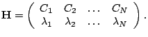
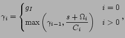
![$\displaystyle \Omega_i=\sum_{k=1}^{i}\Bigl[\gamma_{k-1}\mathbf{x}\Gamma_{k,i}
\Bigr].$](img69.png)
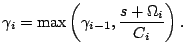
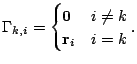
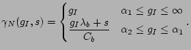
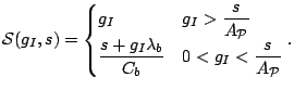
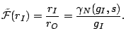
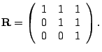
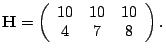
![\includegraphics[width=3.0in]{crfg.eps}](img123.png)
![\includegraphics[width=3.0in]{crfr.eps}](img124.png)
![$\displaystyle \lim_{\delta \rightarrow \infty} E\left[\Bigl(
Y_{i,\delta}(\mathbf{f}_j)-x_j\Bigr)^2 \right]=0.$](img139.png)
![$\displaystyle \lim_{\delta \rightarrow \infty} E\left[\Bigl(
Y_{i,\delta}(\mathbf{p})-\mathbf{x}\mathbf{p}\Bigr)^2 \right]=0.$](img155.png)
![$\displaystyle \lim_{ \delta \rightarrow \infty}E\left[\Bigl(B_{i,\delta}(\mathbf{p})-\left(C_i-\mathbf{xp}\right)\Bigr)^2\right]=0.$](img161.png)
![$\displaystyle \lim_{ \delta \rightarrow\infty}E\left[\Bigl(D_{i,\delta}(\mathbf{p})-0\Bigr)^2\right]=2Var\left[W_i(\mathbf{p})\right].$](img163.png)
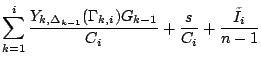
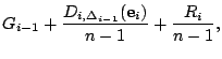
![$\displaystyle E[G_i] \ge \dfrac{1}{C_i}\left(\sum_{k=1}^{i}\mathbf{x}\Gamma_{k,i}E[G_{k-1}]+s \right).$](img209.png)
![$\displaystyle E[G_i]\ge \max\left(E[G_{i-1}], \dfrac{\sum_{k=1}^{i}\mathbf{x}\Gamma_{k,i}E[G_{k-1}]+s}{C_i}\right).$](img210.png)
![$\displaystyle \max\Bigl(E[G_{N-1}],\dfrac{\sum_{k=1}^{N}\mathbf{x}\Gamma_{k,N}
E[G_{k-1}]+s}{C_N}\Bigr)$](img219.png)
![$\displaystyle \beta_i=\begin{cases}
\beta_{i-1}+\dfrac{E[R_i]}{n-1} & \gamma_i...
...beta_{k-1}+\dfrac{E[\tilde{I}_i]}{n-1}
& \gamma_i > \gamma_{i-1}
\end{cases}.$](img224.png)
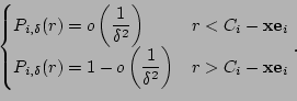
![$\displaystyle \lim_{s\rightarrow \infty}
E\left[G_N\left(\dfrac{s}{r_I}
,s,n\right)-\gamma_N\left(\dfrac{s}{r_I},s\right)\right]=0.$](img232.png)
![$\displaystyle \lim_{s\rightarrow
\infty}E\left[\left(G_N\left(\dfrac{s}{r_I},s,n\right)-\gamma_N\left(\dfrac{s}{r_I},s\right)\right)^2\right]\le
K_N.$](img234.png)
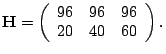
![\includegraphics[width=3.0in]{exp1_rc.eps}](img252.png)
![\includegraphics[width=3.0in]{exp2_rc.eps}](img253.png)
![\includegraphics[width=3.0in]{lulea_cmu.eps}](img270.png)
![\includegraphics[width=3.0in]{pn3.eps}](img271.png)
![\includegraphics[width=2.5in]{elastic.eps}](img278.png)