James Lee Hafner IBM Almaden Research Center hafner@almaden.ibm.com
It has become increasingly clear in the storage industry that RAID5 does not provide sufficient reliability against loss of data either because of multiple concurrent disk losses or disk losses together with sector losses (e.g., due to medium errors from the disks). The reasons are primarily due to the dramatic increase in single disk capacity together with a fairly constant per-bit error rate. Additional factors, as mentioned in [5], include increasing number of disks per system, and use of less reliable disks such as ATA (vs. SCSI). The cited paper makes the case for double fault tolerance; by extrapolation, there is (or will be) a need for higher fault tolerant codes if these trends continue. Furthermore, as the industry moves into very long-term archival storage or dRAID (distributed Redundant Arrangement of Independent Devices) node-based systems, the need for higher fault-tolerance erasure codes will likely become more acute.
![]() -way mirroring can clearly be used to provide additional redundancy
in any system, but the storage efficiency (ratio of user data to the
total of user data plus redundancy data) of mirroring is very low.
(We prefer the term ``efficiency'' in storage contexts instead of the
equivalent term ``rate'' which is more suitable for communication
channels.) On the other hand, codes like Reed-Solomon
(RS) [14] provide optimal storage efficiency (that is,
are maximum distance separable, or MDS) and arbitrarily high fault
tolerance, but require special purpose hardware to enable efficient
computation of the finite field arithmetic on which the codes are
based (or, if formulated as a binary XOR code, generally have higher
computational costs and complexities).
-way mirroring can clearly be used to provide additional redundancy
in any system, but the storage efficiency (ratio of user data to the
total of user data plus redundancy data) of mirroring is very low.
(We prefer the term ``efficiency'' in storage contexts instead of the
equivalent term ``rate'' which is more suitable for communication
channels.) On the other hand, codes like Reed-Solomon
(RS) [14] provide optimal storage efficiency (that is,
are maximum distance separable, or MDS) and arbitrarily high fault
tolerance, but require special purpose hardware to enable efficient
computation of the finite field arithmetic on which the codes are
based (or, if formulated as a binary XOR code, generally have higher
computational costs and complexities).
Other erasure codes have been proposed for better fault tolerance than
RAID5, but none has emerged as a clear winner even in the RAID
controller market - the industry has not even settled on a de
facto standard for ![]() fault tolerance after 40+ years (since RS
codes were first proposed). We believe no such ``perfect'' code can
exist; every code requires some trade-offs in efficiency, performance
or fault tolerance.
fault tolerance after 40+ years (since RS
codes were first proposed). We believe no such ``perfect'' code can
exist; every code requires some trade-offs in efficiency, performance
or fault tolerance.
In this paper, we present the WEAVER codes, so called because the parity/redundancy values are computed by XOR formulas defined by patterns that weave through the data. There are three design principles that characterize WEAVER codes: (a) every strip (stripe unit) contains both data and parity from the same stripe (we call these vertical codes because data and parity are arranged together vertically on each strip), (b) the number of data values that contribute to each parity value (parity in-degree) is fixed and, most importantly, is independent of the stripe size (number of strips) and (c) balance and symmetry. The second property enables flexibility in choices of stripe sizes without altering computational costs (in both XOR and IO). In addition, it bounds the computational costs of many operations (e.g., short writes, rebuild). More details on these points are given in Section 3 and elsewhere.
The WEAVER codes are designed with balance and symmetry in three aspects. First, every parity is constructed from some fixed number of data values (we call this number the ``parity in-degree'' - as noted, it is independent of the stripe size). Second, each data value contributes to a fixed number of parity values (we call this the ``data out-degree''; it is also independent of the stripe size). The data out-degree for WEAVER codes is set to the fault tolerance, the theoretical minimum number for the given fault tolerance. For additional symmetry, some of the codes have the parity in-degree equal to the data out-degree - this provides a certain duality between data and parity. Third, all the code constructions are specified by a weave-pattern which is repeated by simple rotation of a base configuration. That is, they are rotationally symmetric.
We bound the parity in-degree by the fault tolerance to control the complexity of parity computations and improve other properties such as localization (see Section 3.1.2). There are undoubtedly other whole families of codes yet to be discovered that relax this requirement, while keeping the parity in-degree fixed (some Wiencko codes [15,6] may have this property as well).
There are two general families and one ad-hoc family of WEAVER codes,
which we describe in detail later. We briefly mention here that there
are constructions of WEAVER codes that tolerate up to ![]() device
failures (and perhaps beyond). A key feature of all WEAVER codes is
the ``localization'' property that for large stripe sizes limits the
scope of most operations (including, for example, rebuild) to small
subsets of the stripe. This is discussed in more detail in
Section 3.1.2.
device
failures (and perhaps beyond). A key feature of all WEAVER codes is
the ``localization'' property that for large stripe sizes limits the
scope of most operations (including, for example, rebuild) to small
subsets of the stripe. This is discussed in more detail in
Section 3.1.2.
The WEAVER codes are in general not MDS codes (though some
special cases are). Consequently, the main disadvantage of these
codes is their storage efficiency. However, these codes are optimally
efficient for the given fault tolerance and parity in-degree
constraint (see Section 3.2). Of the three
families of WEAVER codes, one family has efficiency 50% for all
levels of fault tolerance (up to ![]() in our constructions); the other
families have lower efficiency which decreases with increasing fault
tolerance. In all cases, these codes have significantly higher
efficiency than
in our constructions); the other
families have lower efficiency which decreases with increasing fault
tolerance. In all cases, these codes have significantly higher
efficiency than ![]() -way mirroring. The WEAVER codes, by their
symmetry, have a certain simplicity of implementation (though not as
simple as
-way mirroring. The WEAVER codes, by their
symmetry, have a certain simplicity of implementation (though not as
simple as ![]() -way mirroring). As such these codes provide a way for a
system designer to select highly fault tolerant codes that interpolate
between
-way mirroring). As such these codes provide a way for a
system designer to select highly fault tolerant codes that interpolate
between ![]() -way mirroring with its performance advantages, exceptional
simplicity but minimal efficiency and MDS codes with somewhat lower
performance and somewhat greater complexity but optimal efficiency.
-way mirroring with its performance advantages, exceptional
simplicity but minimal efficiency and MDS codes with somewhat lower
performance and somewhat greater complexity but optimal efficiency.
Unfortunately, we do not have many theoretical results concerning specific constructions. Generally, for small fault tolerance, these codes can be tested by hand (in some cases, we give the proof). For other cases, our constructions were tested by computer program using the generator matrix (see Section 4 and [10] for related methodology).
The paper is organized as follows. We close this introduction with some definitions and notation. In Section 2 we describe the various constructions for each family of WEAVER codes. Section 3 lists the key advantages and disadvantages of these codes. Related work and comparisons with other published codes are discussed in detail in Section 5. Section 4 outlines our testing methodology. We conclude with a short summary.
The literature contains some inconsistency concerning the use of common storage and erasure code terms, so we state our definitions here to avoid confusion. We use the term ``system'' to refer to either a dRAID storage system of node-type devices or to a controller array of disks (RAID). The term ``device'' will refer to the ``independent'' storage device in the system (a node in dRAID or a disk in RAID).
We use the symbol ![]() exclusively to represent the fault tolerance of
a code, the symbol
exclusively to represent the fault tolerance of
a code, the symbol ![]() for the size of the stripe (the number of
strips, or equivalently, the number of devices in a code instance),
and
for the size of the stripe (the number of
strips, or equivalently, the number of devices in a code instance),
and ![]() for the maximum parity in-degree. For WEAVER codes, all
parity have in-degree exactly
for the maximum parity in-degree. For WEAVER codes, all
parity have in-degree exactly ![]() and
and ![]() . In addition, all data
have out-degree equal to
. In addition, all data
have out-degree equal to ![]() . We therefore parameterize our codes as
WEAVER(
. We therefore parameterize our codes as
WEAVER(![]() ,
,![]() ,
,![]() ), and we provide constructions for different values
of these parameters. We let
), and we provide constructions for different values
of these parameters. We let ![]() denote the number of data elements
and
denote the number of data elements
and ![]() the number of parity elements per strip. (We see how
the number of parity elements per strip. (We see how ![]() and
and
![]() may be determined from
may be determined from ![]() and
and ![]() in Section 2.)
in Section 2.)
We define a ``short write'' as a host write to any sequential subset of an element (e.g., a single sector); a ``multiple strip write'' as a host write to a sequential subset of the strips in a stripe (that is, the user data portion of the strips). The ``write lock zone'' is the set of elements that should be locked during a short write so as to provide data/parity consistency in case of failures encountered during a write operation. The ``rebuild zone'' is the subset of strips within the stripe which are needed during a rebuild of one or more lost strips. We see why these notions are relevant to WEAVER codes in Section 3.
In this section we describe our WEAVER constructions. We use a graph representation to visualize the constrained parity-in degree and fixed data-out degree. A table format is used to visualize the data and parity layout on strips (and so devices). Formulas for ``parity defining sets'' (see below) are used to precisely define each construction. Each of these presentations exhibit some of the balance and symmetry of the WEAVER codes.
Figure 1 shows a directed, bipartite graphical
representation of a general WEAVER code; the nodes on top represent
the data elements in the stripe and the nodes on the bottom represent
the parity elements. An edge connects a data element to a parity
element if that data element contributes to the parity value
computation (we say that the data element ``touches'' this parity
element). For WEAVER(![]() ,
,![]() ,
,![]() ) codes, each data element has data
out-degree equal to
) codes, each data element has data
out-degree equal to ![]() . In addition, each parity element has parity
in-degree exactly
. In addition, each parity element has parity
in-degree exactly ![]() , where
, where ![]() . As mentioned, this constraint
is the key to many of the good properties of these codes.
. As mentioned, this constraint
is the key to many of the good properties of these codes.
![\includegraphics[width=\graphicwidth,bb=70 180 560 540]{figs/WeaverGraph3}](img20.png)
|
Generally, a graphical representation like that of Figure 1 can be used for any XOR-based erasure code (for example, see the Tornado codes [11]). In addition, Tanner graphs may also be used (see the description of the Low-Density Parity-Check codes in [13,12]). In Tanner graphs the nodes on one side represent data and parity and the opposite nodes represent parity checks. The systematic and regular nature of our WEAVER codes makes the Tanner representation less useful for visualization. We use our graphs to show the encoding of data/parity relations, and not for decoding as in [11]. We also draw our graph with nodes on top and bottom (not left/right) to suggest a relationship to the data/parity layout onto strips as described next.
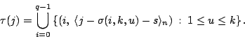
Figure 1 only provides a partial description of the code in the context of storage systems. The physical layout of data and parity on the strips within the stripe must also be specified. This is given in Figure 2 where we see the vertical nature of the WEAVER codes. As noted, other codes share this vertical layout (see, for example, the X-code [17] and the BCP code [1]). We view the logical addressing of the data elements from the host's viewpoint as first within a strip and then strip to strip.
 |
Of course, there is no requirement that the parity elements be placed below the data elements; they must be placed however on the same device. WEAVER codes always have both data and parity elements on each strip. Essential for performance is that the data elements be logically contiguous, as must the parity elements.
We can also represent our codes by sets of indices. A parity element
![]() can be relabeled
can be relabeled
![]() where
where ![]() is
the set of (ordered pair) indices of the data elements that touch this
parity element, That is,
is
the set of (ordered pair) indices of the data elements that touch this
parity element, That is,
For notation, define for any set of ordered pairs of indices ![]() and any offset
and any offset ![]() , a new set of indices referred to as
, a new set of indices referred to as ![]() using the operation
using the operation
Using this notation, we provide rotational symmetry (a key design
feature of WEAVER codes). For ![]() and
and ![]() , set
, set
By counting edges in two ways, it is easy to see from
Figures 1 and 2 that
![]() . Generally, a WEAVER(
. Generally, a WEAVER(![]() ,
,![]() ,
,![]() ) code will have
) code will have ![]() and
and ![]() minimal (to minimize overall complexity): so
minimal (to minimize overall complexity): so ![]() and
and ![]() where
where
![]() . This is assumed throughout unless otherwise noted.
. This is assumed throughout unless otherwise noted.
Given these parameters, the storage efficiency for these codes is
given by
In the next few subsections, we describe specific constructions of parity defining sets that provide for prescribed fault tolerance.
For our first family of WEAVER codes we set ![]() so that efficiency
is 50%. We have
so that efficiency
is 50%. We have ![]() so that
so that ![]() and the layout of
Figure 2 has only one row of data and one row of
parity (see the example below). For this family of codes, we suppress
the first component of each index pair and refer to our parity
defining sets simply as
and the layout of
Figure 2 has only one row of data and one row of
parity (see the example below). For this family of codes, we suppress
the first component of each index pair and refer to our parity
defining sets simply as
![]() for
for ![]() .
We use the following additional notation. Let
.
We use the following additional notation. Let ![]() be an
increasing sequence of
be an
increasing sequence of ![]() integers with initial value
integers with initial value ![]() and let
and let ![]() be an ``offset''. We can specify a parity defining set
be an ``offset''. We can specify a parity defining set ![]() from
from ![]() and
and ![]() by the relation
by the relation
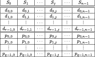
For example, with
![]() and
and ![]() (see
Table 1,
(see
Table 1, ![]() , second entry), the following
diagram provides a valid WEAVER code provided
, second entry), the following
diagram provides a valid WEAVER code provided ![]() .
.
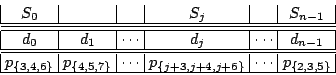
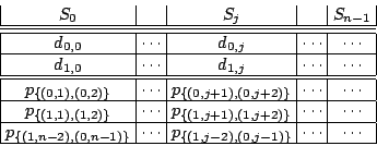
Table 1 gives a partial listing of parity defining
sets (![]() and offset
and offset ![]() ) and valid stripe sizes
) and valid stripe sizes ![]() for
fault tolerance
for
fault tolerance ![]() . (We say a stripe size is ``valid''
for a given parity defining set if the code on that stripe size has
the required fault tolerance.) The entries tagged with an asterisk
are discussed in the remarks below.
. (We say a stripe size is ``valid''
for a given parity defining set if the code on that stripe size has
the required fault tolerance.) The entries tagged with an asterisk
are discussed in the remarks below.
We make the following remarks concerning Table 1.
Consider the ![]() element from Table 1 where
element from Table 1 where
![]() (and
(and ![]() ). We will describe this
code in somewhat different terms and prove the claimed fault
tolerance. With
). We will describe this
code in somewhat different terms and prove the claimed fault
tolerance. With ![]() , each parity value is the XOR sum of a
pair of data values, one from each of the two strips immediately to
the right of the parity element (with wrap-around, of course).
Alternatively, each data element touches two parity elements and so is
paired with two other data elements (the other data element in each of
its two parity elements). From this viewpoint, a given data element
, each parity value is the XOR sum of a
pair of data values, one from each of the two strips immediately to
the right of the parity element (with wrap-around, of course).
Alternatively, each data element touches two parity elements and so is
paired with two other data elements (the other data element in each of
its two parity elements). From this viewpoint, a given data element
![]() is paired with its west
is paired with its west ![]() and east
and east ![]() neighbor elements
(graphically):
neighbor elements
(graphically):
We now give a proof that this code has the required ![]() fault
tolerance, provided
fault
tolerance, provided ![]() . It is clear that this is a necessary
condition (if
. It is clear that this is a necessary
condition (if ![]() and two strips are lost, there is at most only
one strip remaining and that is clearly insufficient). It is also
clear that we only need to recover lost data values, as parity values
can be recomputed from all the data.
and two strips are lost, there is at most only
one strip remaining and that is clearly insufficient). It is also
clear that we only need to recover lost data values, as parity values
can be recomputed from all the data.
There are three cases to consider.
Case 1: Suppose one strip is lost (say, strip ![]() ). We observe
that
). We observe
that
![]() so that
so that ![]() can be recovered by reading
can be recovered by reading
![]() (from the strip
(from the strip ![]() to the right of strip
to the right of strip ![]() ),
reading
),
reading
![]() (from the strip
(from the strip ![]() to the left of
to the left of
![]() ), and using the formula:
), and using the formula:
Case 2: If two adjacent strips are lost (say, ![]() and
and
![]() ), we read
), we read ![]() and
and
![]() (in one operation
from strip
(in one operation
from strip ![]() ) and
) and
![]() from
from ![]() . Then,
recursively,
. Then,
recursively,
Case 3: If two non-adjacent strips are lost, then we
reconstruct as two independent cases of a single strip loss
(using (5)), because the data can always be
reconstructed from its left neighboring parity and right neighboring
data (neither of which is on a lost strip). For ![]() ,
most of the dual failure cases are of this type.
,
most of the dual failure cases are of this type.
In this proof, we saw two examples of the ``localization'' property of
WEAVER codes (see Section 3.1.2). For all cases,
only a few devices in the stripe need to be accessed for
reconstruction; this number is independent of the stripe size ![]() . In
addition, in Case 3 the reconstruction problem split into two
smaller, easier and independent reconstruction problems.
. In
addition, in Case 3 the reconstruction problem split into two
smaller, easier and independent reconstruction problems.
We also saw how the vertical layout reduces device access costs, by combining some multi-element reads into a single device access. For disk arrays, this implies fewer disk seeks and better performance.
The constructions of the previous section are ``ad hoc''; that is,
(with the exception of the case ![]() ) they were found by computer
search and not by a parametric formulation of the parity defining sets
) they were found by computer
search and not by a parametric formulation of the parity defining sets
![]() . In this section, we give a different and formulaic
construction.
. In this section, we give a different and formulaic
construction.
We start by making the assumption that ![]() divides
divides ![]() . Then
. Then
![]() so we can take
so we can take ![]() (one data row) and
(one data row) and ![]() (
(![]() parity rows). We use the term consecutive-
parity rows). We use the term consecutive-![]() to mean consecutive
numbers with difference
to mean consecutive
numbers with difference ![]() . (For example, the consecutive-
. (For example, the consecutive-![]() numbers starting at
numbers starting at ![]() are
are ![]() .) We say a set of parity
elements are consecutive-
.) We say a set of parity
elements are consecutive-![]() if they are in the same row and their
corresponding strip numbers are consecutive-
if they are in the same row and their
corresponding strip numbers are consecutive-![]() , modulo
, modulo ![]() .
.
The constructions are described as follows. In parity row ![]() , data
element
, data
element ![]() touches
touches ![]() consecutive-
consecutive-![]() parity elements to the left,
ending at some left-offset
parity elements to the left,
ending at some left-offset ![]() from
from ![]() (with wrap-around). In each
parity row
(with wrap-around). In each
parity row ![]() ,
, ![]() , data element
, data element ![]() touches the set of
touches the set of
![]() consecutive-
consecutive-![]() parity elements ending one strip to the left
of the first parity element touched in the previous row (again, with
wrap-around). A data element touches exactly
parity elements ending one strip to the left
of the first parity element touched in the previous row (again, with
wrap-around). A data element touches exactly ![]() parity elements in
each row so that each parity is composed of
parity elements in
each row so that each parity is composed of ![]() data elements (that
is, parity in-degree is
data elements (that
is, parity in-degree is ![]() ).
).
Figure 3 shows a graph representation for the special
case when ![]() ,
, ![]() and so
and so ![]() and
and ![]() . This graph is that
subgraph of the general graph in Figure 1
corresponding to the out-edges for the one data element
. This graph is that
subgraph of the general graph in Figure 1
corresponding to the out-edges for the one data element ![]() (and by
rotational symmetry, implies the subgraph for all other data
elements).
(and by
rotational symmetry, implies the subgraph for all other data
elements).
![\includegraphics[width=\graphicwidth,bb=68 188 546 532]{figs/WeaverMultirow3}](img169.png)
|
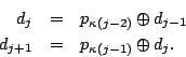
Put in mathematical terms, the set
![]() of (ordered
pairs of) indices of parity elements touched by
of (ordered
pairs of) indices of parity elements touched by ![]() is given
by the formula
is given
by the formula
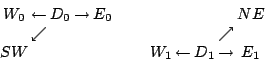
Table 2 provides a list of some examples found by
testing all ![]() and all
and all ![]() for
for ![]() and
and ![]() for
for
![]() . We also give the efficiency,
. We also give the efficiency,
![]() by (4); in the previous section, all codes had
efficiency 50%. Notice the examples with fault tolerance as high
as
by (4); in the previous section, all codes had
efficiency 50%. Notice the examples with fault tolerance as high
as ![]() . We conjecture that this construction (with a suitable
offset
. We conjecture that this construction (with a suitable
offset ![]() and sufficiently large
and sufficiently large ![]() ) should work for arbitrarily
large
) should work for arbitrarily
large ![]() , though not necessarily all
, though not necessarily all ![]() .
.
|
The examples with ![]() and
and ![]() are interesting because the
fault tolerances are so high, but the efficiency is 250% higher and
325% higher than corresponding
are interesting because the
fault tolerances are so high, but the efficiency is 250% higher and
325% higher than corresponding ![]() -way or
-way or ![]() -way mirrors. The two
examples in Table 2 with
-way mirrors. The two
examples in Table 2 with ![]() and
and ![]() are
identical to the WEAVER(
are
identical to the WEAVER(![]() ,
,![]() ,
,![]() ) codes given in
Table 1 with
) codes given in
Table 1 with
![]() and
and
![]() , respectively.
, respectively.
There are two codes in Table 2 with the same fault
tolerance ![]() ; they have different parity in-degree
; they have different parity in-degree ![]() and so
different efficiency. The code with
and so
different efficiency. The code with ![]() has very simple parity
computations but efficiency only 25%. The code with
has very simple parity
computations but efficiency only 25%. The code with ![]() has
somewhat more complex parity computations but better efficiency 33%.
This exemplifies one of the trade-offs of erasure codes (performance
vs. efficiency) and the fact that the rich set of WEAVER codes provide
a means to balance these trade-offs for a given system's constraints.
(Similar remarks apply to the three codes with
has
somewhat more complex parity computations but better efficiency 33%.
This exemplifies one of the trade-offs of erasure codes (performance
vs. efficiency) and the fact that the rich set of WEAVER codes provide
a means to balance these trade-offs for a given system's constraints.
(Similar remarks apply to the three codes with ![]() .)
.)
The remark made in the comments of Section 2.1
about consecutive parity elements when ![]() precludes this
construction from working for
precludes this
construction from working for ![]() . For
. For ![]() and
and ![]() the
situation is undecided. Preliminary experiments suggest that
the
situation is undecided. Preliminary experiments suggest that ![]() suffers from a similar obstacle; surprisingly
suffers from a similar obstacle; surprisingly ![]() does have some
valid configurations. Clearly, alternatives to consecutive-
does have some
valid configurations. Clearly, alternatives to consecutive-![]() may be
required if
may be
required if ![]() (though we have not tested any of these cases).
(though we have not tested any of these cases).
There is considerably more structure to the patterns of valid offsets and stripe sizes for this construction compared to those of the previous section. It is likely that this construction can be analyzed in most cases theoretically. We conjecture that other parity defining sets will also provide valid WEAVER codes of similar efficiency and design, perhaps on even smaller stripe sizes or will fill in the gaps in the stripe sizes in Table 2. We leave these two issues to future work.
The constructions we have presented so far have one data row (![]() ,
because
,
because ![]() divides
divides ![]() in all cases). In the next two sections, we
give two ad-hoc constructions (with
in all cases). In the next two sections, we
give two ad-hoc constructions (with ![]() and
and ![]() fault tolerance,
respectively) that have
fault tolerance,
respectively) that have ![]() . The key feature of these codes is that
we restrict
. The key feature of these codes is that
we restrict ![]() , so that the parity computations are quite simple.
, so that the parity computations are quite simple.
These codes generalize the ![]() fault tolerant code discussed in
Section 2.1.1. They each contain two copies of this
fault tolerant code discussed in
Section 2.1.1. They each contain two copies of this
![]() fault tolerant code, plus some additional cross relations between
them (hence, again the WEAVER name). All three codes use ``data
neighbor'' relations to determine the parity defining sets. Adding a
second row allows for relations in different directions than just
east/west; this in turn enables more parity defining sets containing a
given data element; and this increases the (potential) fault
tolerance.
fault tolerant code, plus some additional cross relations between
them (hence, again the WEAVER name). All three codes use ``data
neighbor'' relations to determine the parity defining sets. Adding a
second row allows for relations in different directions than just
east/west; this in turn enables more parity defining sets containing a
given data element; and this increases the (potential) fault
tolerance.
The WEAVER(![]() ,
,![]() ,
,![]() ) code presented in this section has a
data/parity layout given by
) code presented in this section has a
data/parity layout given by
Visually, data elements ![]() from the first row and
from the first row and ![]() from the
second row are paired with neighbors as in the following diagram (each
pair computes a different parity value):
from the
second row are paired with neighbors as in the following diagram (each
pair computes a different parity value):
It can be proven that this construction is also sufficient for ![]() fault tolerance provided
fault tolerance provided ![]() but we leave out the proof as it is
similar to the one we gave for WEAVER(
but we leave out the proof as it is
similar to the one we gave for WEAVER(![]() ,
,![]() ,
,![]() ).
).
This construction provides another example of a ![]() fault tolerant
code on as few as
fault tolerant
code on as few as ![]() devices. Compare this with the first
devices. Compare this with the first ![]() entry in Table 1 where
entry in Table 1 where ![]() ; the difference is
again a performance/efficiency trade-off. See
Section 5 for more comments.
; the difference is
again a performance/efficiency trade-off. See
Section 5 for more comments.
In this section we provide another WEAVER(![]() ,
,![]() ,
,![]() ) code with two
data rows. Contrast this construction with the code of
Section 2.2, which also has
) code with two
data rows. Contrast this construction with the code of
Section 2.2, which also has ![]() and
and ![]() but has only one data row (see Table 2). This is the
only code we present that drops the ``minimalist'' condition
but has only one data row (see Table 2). This is the
only code we present that drops the ``minimalist'' condition
![]() .
.
The layout and parity defining sets can be seen in the following chart:
This time, each data element is paired with four other data elements:
west, east, and two diagonal neighbors (southwest, southeast for an
element ![]() in row
in row ![]() and northeast, northwest for a an element
and northeast, northwest for a an element ![]() in row
in row ![]() ). Graphically, this looks like:
). Graphically, this looks like:
Again, we leave out the proof that this is ![]() fault tolerant provided
fault tolerant provided
![]() . This code has the same fault tolerance, efficiency and
parity in-degree as the WEAVER(
. This code has the same fault tolerance, efficiency and
parity in-degree as the WEAVER(![]() ,
,![]() ,
,![]() ) code in
Table 2, but requires more strips for the minimal
configuration (and has six rows in total versus three for the previous
code). However, it has better localization properties. For example,
for this construction the write lock zone comprises a total of eight
data and parity elements on six neighboring strips (centered on the
target strip) versus the same number of data and parity elements on
seven strips (five neighboring strips similarly centered plus two
additional strips) for the
) code in
Table 2, but requires more strips for the minimal
configuration (and has six rows in total versus three for the previous
code). However, it has better localization properties. For example,
for this construction the write lock zone comprises a total of eight
data and parity elements on six neighboring strips (centered on the
target strip) versus the same number of data and parity elements on
seven strips (five neighboring strips similarly centered plus two
additional strips) for the ![]() code of
Section 2.2.
code of
Section 2.2.
Note that by dropping the first two rows of parity, we get yet another
WEAVER(![]() ,
,![]() ,
,![]() ) code with two data rows, two parity rows and
efficiency 50%. It can be made equivalent to the code described in
Section 2.1.1 and so is not very interesting by itself.
) code with two data rows, two parity rows and
efficiency 50%. It can be made equivalent to the code described in
Section 2.1.1 and so is not very interesting by itself.
Now that we have defined the WEAVER codes and given many examples, we next discuss the key features of these codes, the advantages in the next subsection and a brief discussion of the primary disadvantage following.
The WEAVER codes have instances of exceptionally high fault tolerance
(we gave constructions with fault tolerance ![]() and conjecture that
other constructions should be possible). There are few codes in the
storage system literature that meet these fault tolerance levels. The
only viable options for very high fault tolerance to date seem to be
Reed-Solomon codes, with their high computational costs, or
and conjecture that
other constructions should be possible). There are few codes in the
storage system literature that meet these fault tolerance levels. The
only viable options for very high fault tolerance to date seem to be
Reed-Solomon codes, with their high computational costs, or ![]() -way
mirroring with their very low efficiency. See also the remarks in
Section 5 on the LDPC and Wiencko codes.
-way
mirroring with their very low efficiency. See also the remarks in
Section 5 on the LDPC and Wiencko codes.
The design characteristics of constant parity in-degree and rotational symmetry are key features of the WEAVER codes. They enable the ``localization'' of many operations on the stripe. We have seen two examples of this: (a) in Section 2.1.1 we saw reconstruction requiring access to a small bounded (independent of stripe size) subset of the stripe; and (b) in Section 2.3.2 we saw write lock zones for two codes that are also small, bounded subsets of the stripe.
These two examples are typical of any WEAVER code (in fact, any code
with parity in-degree bounded independent of the stripe size). The
write lock zone (see Section 1.1) can be determined by
examining the 2-neighborhood of the target element in the data/parity
graph (see Figure 1 - the 2-neighborhood is the
set of nodes in the graph within a distance two of the target
element's node). With ![]() parities each having
parities each having ![]() out edges (one of
which is the target element), this bounds the write lock zone to at
most
out edges (one of
which is the target element), this bounds the write lock zone to at
most ![]() data and parity elements (so at most
data and parity elements (so at most ![]() devices
as well - for some WEAVER codes, the actual number of devices is
smaller). This is independent of the stripe size
devices
as well - for some WEAVER codes, the actual number of devices is
smaller). This is independent of the stripe size ![]() , providing a
proof of the localized write lock zone.
, providing a
proof of the localized write lock zone.
In contrast, even RAID5 has a write lock zone that is effectively the entire stripe, since the 2-neighborhood of an element is the entire remainder of the stripe. This is a consequence of the parity in-degree determined as a function of the stripe size.
Similar localization effects occur during rebuild. A rebuild of one
or more lost strips in a WEAVER code only requires access to a fixed
and bounded set of strips. This set is at most the union of the
2-neighborhoods for all the data elements on all the lost strips (and
is independent of ![]() as well). Also, as we saw in
Section 2.1.1, certain multi-strip failures may partition
themselves into independent smaller failure scenarios. Reconstruction
algorithms generally get more complicated with the number of
inter-related failures so partitioning a multiple failure case into
two or more independent failure cases can have a significant
performance advantage and enable parallelism. For example, consider
the recovery costs of EVENODD(
as well). Also, as we saw in
Section 2.1.1, certain multi-strip failures may partition
themselves into independent smaller failure scenarios. Reconstruction
algorithms generally get more complicated with the number of
inter-related failures so partitioning a multiple failure case into
two or more independent failure cases can have a significant
performance advantage and enable parallelism. For example, consider
the recovery costs of EVENODD(![]() ,
,![]() ) [2] and
WEAVER(
) [2] and
WEAVER(![]() ,
,![]() ,
,![]() ) code when two strips fail. For
) code when two strips fail. For ![]() , the
EVENODD always requires accessing
, the
EVENODD always requires accessing ![]() devices, whereas most cases of
WEAVER recovery involve only 4 devices, and the other cases only
require 2 devices to be accessed!
devices, whereas most cases of
WEAVER recovery involve only 4 devices, and the other cases only
require 2 devices to be accessed!
The vertical layout of data and parity together with the symmetry properties (balanced parity in-degree and data out-degree and the rotational pattern) provide natural load balancing across all the devices. Multiple instances of the WEAVER codes can be stacked on the same set of devices with a simple host-to-strip addressing and also a simple logical strip-to-physical-device labeling. In contrast, the parity rotation of RAID5 vs RAID4 requires more complicated logical/physical addressing models.
Furthermore, multiple WEAVER code instances with different fault tolerances can be easily stacked on the same collection of devices (provided the number of devices is sufficiently large). This enables different reliability classes of logical volumes on the same set of devices. This is possible with other codes, but generally requires more complex logical/physical addressing.
The localization property mentioned above enables the WEAVER stripes
to be expanded or shrunk with only local effects to the stripe; that
is, not all devices need to be accessed and data or parity moved
around. For example, in the WEAVER(![]() ,
,![]() ,
,![]() ) codes, new
devices/strips can be inserted into the stripe, and only the nearby
devices need to have parity recomputed. See the additional comments
in Section 5.
) codes, new
devices/strips can be inserted into the stripe, and only the nearby
devices need to have parity recomputed. See the additional comments
in Section 5.
With the WEAVER(![]() ,
,![]() ,
,![]() ) codes, it is further possible to change,
on-the-fly, the fault tolerance of a single stripe in the system
(either up or down) by simply recomputing the parity values. No
remapping of either the host addressing or the strip labeling is
needed. The only requirement is that the stripe size is supported for
the higher fault tolerance. This enables more autonomic adaptability
and is not possible with (almost) any other code. In addition, by
using a chain of
) codes, it is further possible to change,
on-the-fly, the fault tolerance of a single stripe in the system
(either up or down) by simply recomputing the parity values. No
remapping of either the host addressing or the strip labeling is
needed. The only requirement is that the stripe size is supported for
the higher fault tolerance. This enables more autonomic adaptability
and is not possible with (almost) any other code. In addition, by
using a chain of ![]() subsets (e.g., those marked by a
asterisk in Table 1), the recomputation step
involves only adding a single new data value into each parity value
and then storing the new parity values in the appropriate strips (which
changes only if the offset changes). This is significantly more
efficient than recomputing all the parity from scratch. Note that
``adding a data value'' can be used to either lower or raise the fault
tolerance.
subsets (e.g., those marked by a
asterisk in Table 1), the recomputation step
involves only adding a single new data value into each parity value
and then storing the new parity values in the appropriate strips (which
changes only if the offset changes). This is significantly more
efficient than recomputing all the parity from scratch. Note that
``adding a data value'' can be used to either lower or raise the fault
tolerance.
We believe that these features in particular make the WEAVER codes
best suited for dRAID (distributed Redundant Arrangement of
Independent Devices) systems involving network-connected storage
nodes. Such systems will likely have data sets with varying
reliability and performance requirements. Such sets may be
distributed across different but intersecting sets of nodes. The
WEAVER variability of stripe size and fault tolerance enable a dRAID
data distribution algorithm to focus on user data layout (e.g., for
load-balancing) and to achieve a balanced parity distribution as a
natural consequence of the code itself. In addition, the chain of
design sets for WEAVER(![]() ,
,![]() ,
,![]() ) codes allows the system to change
fault tolerance with minimal network bandwidth utilization. Each node
reads both its data and parity values, and sends only a single data
value over the network, performs a single XOR operation, sends the
recomputed parity value over the network and then performs a single
disk write operation of the new parity). The parity ``send'' step is
only required if the offset changes; more interestingly, the data
``send'' step may be skipped for some parity defining set subset
chains. This operation is then both load-balanced and disk and
network efficient.
) codes allows the system to change
fault tolerance with minimal network bandwidth utilization. Each node
reads both its data and parity values, and sends only a single data
value over the network, performs a single XOR operation, sends the
recomputed parity value over the network and then performs a single
disk write operation of the new parity). The parity ``send'' step is
only required if the offset changes; more interestingly, the data
``send'' step may be skipped for some parity defining set subset
chains. This operation is then both load-balanced and disk and
network efficient.
For most of the WEAVER(![]() ,
,![]() ,
,![]() ) codes, the short write IO cost in
device accesses (e.g., disk seeks) is equal to
) codes, the short write IO cost in
device accesses (e.g., disk seeks) is equal to ![]() . For the
parity update algorithm that uses the parity delta, this seek cost is
optimal for any
. For the
parity update algorithm that uses the parity delta, this seek cost is
optimal for any ![]() fault tolerant code. Many codes have even higher
short write IO costs, when a given data element touches more than
fault tolerant code. Many codes have even higher
short write IO costs, when a given data element touches more than ![]() parity elements (and strip sizes are large - see
Section 3.1.7). For example, the EVENODD
codes [2,3] have this property for
some elements.
parity elements (and strip sizes are large - see
Section 3.1.7). For example, the EVENODD
codes [2,3] have this property for
some elements.
Furthermore, only codes of efficiency (approximately) 50% can achieve
better short write IO seek costs than the typical ![]() . For
example, a
. For
example, a ![]() -fault tolerant Reed-Solomon code can perform a short
write in
-fault tolerant Reed-Solomon code can perform a short
write in ![]() seeks but only if
seeks but only if ![]() (so efficiency 50%) or in
(so efficiency 50%) or in
![]() seeks only if
seeks only if ![]() (so efficiency close to 50%). In
these cases, the stripe size is fixed as a function of the fault
tolerance
(so efficiency close to 50%). In
these cases, the stripe size is fixed as a function of the fault
tolerance ![]() . Mirroring achieves the best short write IO seek costs
(
. Mirroring achieves the best short write IO seek costs
(![]() ) but also has the lowest efficiency.
) but also has the lowest efficiency.
In contrast, some WEAVER codes achieve better short write IO seek
costs for a given fault tolerance and for any valid stripe size.
For example, the WEAVER(![]() ,
,![]() ,
,![]() ) code (see
Section 2.1.1) enables an implementation of a short write
with
) code (see
Section 2.1.1) enables an implementation of a short write
with ![]() IOs (one less than is typical). This is achieved by reading
the west and east neighbors of the target data element, computing the
two new parities (from the parity equations) and writing the two new
parities and one new data.
IOs (one less than is typical). This is achieved by reading
the west and east neighbors of the target data element, computing the
two new parities (from the parity equations) and writing the two new
parities and one new data.
Similarly, by amortizing two neighbor data element reads into one
longer read, the other two ad hoc WEAVER codes with parity in-degree
equal to ![]() can achieve a short write IO seek cost of
can achieve a short write IO seek cost of ![]() (for fault
tolerance
(for fault
tolerance ![]() , Section 2.3.1) and
, Section 2.3.1) and ![]() (for fault
tolerance
(for fault
tolerance ![]() , Section 2.3.2). We emphasize that these IOs
are not all of the same length, and a fairer comparison should take
this into account (we do not do that here since seeks dominate device
access costs; but see [9] for a more thorough analysis
of these issues).
, Section 2.3.2). We emphasize that these IOs
are not all of the same length, and a fairer comparison should take
this into account (we do not do that here since seeks dominate device
access costs; but see [9] for a more thorough analysis
of these issues).
Many of the WEAVER codes can amortize a significant number of device
accesses required for consecutive multi-strip host writes. We explain
this in detail for the WEAVER(![]() ,
,![]() ,
,![]() ) code
(Section 2.1.1) and leave it to the reader to see how this
principle can be applied in other WEAVER constructions. We will
contrast the WEAVER behavior with EVENODD [2] which is
also 2 fault tolerant, though this analysis applies to many other
2-fault tolerant codes, including Reed-Solomon [14].
) code
(Section 2.1.1) and leave it to the reader to see how this
principle can be applied in other WEAVER constructions. We will
contrast the WEAVER behavior with EVENODD [2] which is
also 2 fault tolerant, though this analysis applies to many other
2-fault tolerant codes, including Reed-Solomon [14].
Suppose the system gets a host write for ![]() consecutive strips in a
stripe of size
consecutive strips in a
stripe of size ![]() . For the EVENODD code, there are two efficient
implementations. The first implementation reads all the
. For the EVENODD code, there are two efficient
implementations. The first implementation reads all the ![]() strips
and the
strips
and the ![]() parity strips, computes the new parity strips and writes
the
parity strips, computes the new parity strips and writes
the ![]() data strips and
data strips and ![]() parity strips for a total of
parity strips for a total of ![]() device
accesses. The second implementation reads the
device
accesses. The second implementation reads the ![]() other
(2-neighborhood) data strips, computes the parity and writes
other
(2-neighborhood) data strips, computes the parity and writes ![]() data and parity strips for a total of
data and parity strips for a total of ![]() device accesses. The
optimum number of device accesses is then
device accesses. The
optimum number of device accesses is then ![]() .
.
In contrast, the following diagram shows how this could be implemented
for a WEAVER(![]() ,
,![]() ,
,![]() ) code. In the diagram, an
) code. In the diagram, an ![]() indicates a
data element that we read (only), a
indicates a
data element that we read (only), a ![]() indicates a data element that
we write (this is a target of the host IO),
indicates a data element that
we write (this is a target of the host IO), ![]() indicates a parity
element that we write (we do not read any parity or old data).
indicates a parity
element that we write (we do not read any parity or old data).
XOR-based erasure codes have typically two alternative implementations with respect to size (number of bytes) that are mapped to each strip. One choice is to map a strip to a small unit of the device, e.g., 512B or perhaps 4KB. In this case, a host short write maps to a full strip write and the parity computations involve all (or most) of the parity elements. Generally, Reed-Solomon codes are implemented as extreme examples of this where a strip is a byte. XOR-based codes may be implemented in this way as well, but multiple rows impose fragmentation of the parity computations.
The alternative is to map a strip to a unit comparable to a moderate size host IO (say, 256KB as is typically done in RAID5). In these cases, elements are much larger units and a host short write affects only a subportion of an element. With this implementation, the host short write costs can scale to larger host IO lengths, up to the size of the element, incurring additional costs that are only linear functions of the length. There are no additional seeks or other computational costs such as additional XOR formulas.
For a fixed strip size, more data rows in the code imply smaller
element size (for a fixed strip size), and hence limitations on the
advantages of this uniform and linear scaling. In this regard, (most
of) the WEAVER codes are optimal because they have only one data row
(the ad hoc constructions have two data rows, so are near optimal).
They also do not suffer from excessive XOR fragmentation for the same
reason. (Clearly, RAID5 and ![]() -way mirroring have these properties
as well but they are at opposite ends of the
fault-tolerance/efficiency spectrum, with WEAVER codes occupying the
middle ground. See Section 5 for additional
comments.)
-way mirroring have these properties
as well but they are at opposite ends of the
fault-tolerance/efficiency spectrum, with WEAVER codes occupying the
middle ground. See Section 5 for additional
comments.)
The primary disadvantage of the WEAVER codes is their limited
efficiency (at most 50%). On the other hand, WEAVER codes are
optimally efficient among all possible codes of fault tolerance ![]() and parity in-degree
and parity in-degree ![]() as the following argument shows.
Suppose an erasure code with fault tolerance
as the following argument shows.
Suppose an erasure code with fault tolerance ![]() has
has ![]() data elements
and
data elements
and ![]() parity elements and that each parity element has parity
in-degree bounded above by
parity elements and that each parity element has parity
in-degree bounded above by ![]() . Each data element must touch at least
. Each data element must touch at least
![]() parity elements. Counting edges in the parity graph (as in the
WEAVER example in Figure 1), we see that the
number of edges
parity elements. Counting edges in the parity graph (as in the
WEAVER example in Figure 1), we see that the
number of edges ![]() is at least
is at least ![]() (counting the edges coming out of
the data nodes) and at most
(counting the edges coming out of
the data nodes) and at most ![]() (counting the edges coming into the
parity nodes); that is,
(counting the edges coming into the
parity nodes); that is, ![]() . The efficiency is
. The efficiency is
We have mentioned above that we search parameter spaces for valid
configurations, that is, configurations that provide the requisite
fault tolerance. Our methodology is the following (see
also [10]). For each fault tolerance ![]() and each
choice of parity defining set (including offset), and for each stripe
size
and each
choice of parity defining set (including offset), and for each stripe
size ![]() , we construct the binary generator matrix for the WEAVER code
of those parameters. This matrix has rows indexed by the data
elements and columns indexed by the data and parity elements. A
column with a single one indicates a data element; a column with at
least 2 ones indicates a parity element (and the formula used to
compute it - that is, the data elements touching it). We view the
generator matrix in column block form where each block corresponds to
a strip; the columns in a block correspond to data and parity elements
on the same strip. The blocks are indexed by the numbers
, we construct the binary generator matrix for the WEAVER code
of those parameters. This matrix has rows indexed by the data
elements and columns indexed by the data and parity elements. A
column with a single one indicates a data element; a column with at
least 2 ones indicates a parity element (and the formula used to
compute it - that is, the data elements touching it). We view the
generator matrix in column block form where each block corresponds to
a strip; the columns in a block correspond to data and parity elements
on the same strip. The blocks are indexed by the numbers
![]() since there are
since there are ![]() strips. The generator matrix
then maps the input user data into data and parity elements, and the
block structure shows how they are organized on strips.
strips. The generator matrix
then maps the input user data into data and parity elements, and the
block structure shows how they are organized on strips.
We can simulate strip loss by removing (or zeroing) the columns of
the corresponding block. Consequently, to test this code for the
required fault tolerance ![]() , we execute the following pseudo-code:
, we execute the following pseudo-code:
For rotationally symmetric codes like the WEAVER codes, one can
restrict the search space a bit by requiring that ![]() . Other
such restrictions may be used to reduce the search space further
(e.g., see [6]).
. Other
such restrictions may be used to reduce the search space further
(e.g., see [6]).
As ![]() and
and ![]() grow, this search space grows rather rapidly, as there
are
grow, this search space grows rather rapidly, as there
are
![]() such cases to consider (and the matrices get
larger as
such cases to consider (and the matrices get
larger as ![]() ).
Other optimizations are possible that reduce these costs.
).
Other optimizations are possible that reduce these costs.
The WEAVER codes can be compared to any other erasure code suitable
for storage systems (we have mentioned some already such as
Reed-Solomon and EVENODD). For ease of comparison, we divide the set
of known erasure codes into different categories and give
(non-exhaustive) examples in each category. In a category by
themselves are the Reed-Solomon codes [14], which are MDS
but require complex finite field arithmetic. Second are XOR-based
codes that are MDS. These come in two types: vertical codes such as
the X-code [17], BCP [1] or ZZS
codes [18] and horizontal codes such as
EVENODD [2,3],
Blaum-Roth [4], or Row-Diagonal Parity
codes [5]. Finally, there are non-MDS codes that
are XOR-based. These subdivide into three categories based on
efficiency: ![]() -way mirroring (trivially XOR-based) with efficiency
less than 50%, the Gibson, et al, codes [8]
with efficiency larger than 50%, and two codes with efficiency 50%
exactly. In the last category, we have the LSI
code [16] (in fact a subcode of one of the
Gibson et al codes) and one
-way mirroring (trivially XOR-based) with efficiency
less than 50%, the Gibson, et al, codes [8]
with efficiency larger than 50%, and two codes with efficiency 50%
exactly. In the last category, we have the LSI
code [16] (in fact a subcode of one of the
Gibson et al codes) and one ![]() fault tolerant Blaum-Roth
binary code [4]. In the second category, we also have the
LDPC codes (see [7,11,13,12]) and
the Wiencko codes [15,6] which we
address separately.
fault tolerant Blaum-Roth
binary code [4]. In the second category, we also have the
LDPC codes (see [7,11,13,12]) and
the Wiencko codes [15,6] which we
address separately.
LDPC codes [7,11] where originally designed for communication channels but have recently been studied in the context of storage applications over wide-area networks [13,12]. In these applications, random packet loss (or delay) is the dominant erasure model (not total device failure), so a typical ``read'' a priori assumes random erasures and hence is always in reconstruction mode. Because of this, good LDPC codes have highly irregular graph structures but can have high fault tolerance and near optimal efficiency (both in the sense of expected value, however). In contrast, the WEAVER codes are designed for a traditional storage model where reads involve reconstruction algorithms only if the direct read the user data fails. In addition, WEAVER codes have very regular graphs, and relatively high fault tolerance over a wide range of stripe sizes.
The Wiencko codes are presented in the patent [15] and patent application [6] as methodologies for formulating and testing a specific code instance code via design patterns. This is similar to the BCP [1] patent. The Wiencko codes are vertical codes (with layout as in Figure 2) and can utilize rotational symmetry. Valid constructions meet certain parameter constraints, and include MDS design possibilities. Few examples are given in these references, however. The construction methodology differs from WEAVER codes in that no a priori restrictions are placed on the parity in-degree. In fact, some examples have differing degree for different parity values; so are less regular and uniform than required in WEAVER codes. Essentially any vertical code such as the X-code [17] and BCP [1] can also be (re)constructed by a Wiencko formulation.
With the exception of the Reed-Solomon codes, ![]() -way mirroring, LDPC
and Wiencko codes, none of the codes have exceptionally high fault
tolerance. There are variations of EVENODD [3]
that are
-way mirroring, LDPC
and Wiencko codes, none of the codes have exceptionally high fault
tolerance. There are variations of EVENODD [3]
that are ![]() fault tolerant; there is one instance of a BCP code
of three fault tolerance on 12 strips; the Blaum-Roth [4]
binary code of efficiency 50% and two codes in [8]
are
fault tolerant; there is one instance of a BCP code
of three fault tolerance on 12 strips; the Blaum-Roth [4]
binary code of efficiency 50% and two codes in [8]
are ![]() fault tolerant. As far as we know, none of the other codes
have variants that can tolerate more than
fault tolerant. As far as we know, none of the other codes
have variants that can tolerate more than ![]() failures. The WEAVER
codes can have very high fault tolerance (up to 12 and perhaps
beyond). Compared to Reed-Solomon codes, they are significantly
simpler but less efficient. Compared to
failures. The WEAVER
codes can have very high fault tolerance (up to 12 and perhaps
beyond). Compared to Reed-Solomon codes, they are significantly
simpler but less efficient. Compared to ![]() -way mirroring, they are
more complex but more efficient. The WEAVER codes provide alternative
interpolating design points between Reed-Solomon and
-way mirroring, they are
more complex but more efficient. The WEAVER codes provide alternative
interpolating design points between Reed-Solomon and ![]() -way mirroring
over a long range of fault tolerances.
-way mirroring
over a long range of fault tolerances.
As we mentioned in Section 3.1.5, only codes with
efficiency approximately 50% can implement a host short write with
fewer IO seeks than ![]() ; the implementation in fact must compute
parity from new data and the 2-neighborhood dependent data. To
achieve IO seeks costs less than
; the implementation in fact must compute
parity from new data and the 2-neighborhood dependent data. To
achieve IO seeks costs less than ![]() , this 2-neighborhood must be
small. Special subcodes of the horizontal codes (both MDS and
non-MDS) can achieve this but only if the stripe size is bounded as a
function the fault tolerance:
, this 2-neighborhood must be
small. Special subcodes of the horizontal codes (both MDS and
non-MDS) can achieve this but only if the stripe size is bounded as a
function the fault tolerance: ![]() or
or ![]() . The
Blaum-Roth [4] three fault tolerant (binary) code is
equivalent to a very special case of Reed-Solomon with
. The
Blaum-Roth [4] three fault tolerant (binary) code is
equivalent to a very special case of Reed-Solomon with ![]() and so
can be implemented with a
and so
can be implemented with a ![]() IO seeks (at efficiency 50%). In these
implementations, the strip size must be comparable to the short write
IO size (see Section 3.1.7) so that a short write
contains a strip. Only the LSI code [16] and the
WEAVER(
IO seeks (at efficiency 50%). In these
implementations, the strip size must be comparable to the short write
IO size (see Section 3.1.7) so that a short write
contains a strip. Only the LSI code [16] and the
WEAVER(![]() ,
,![]() ,
,![]() ) codes support variable stripe sizes of fixed fault
tolerance and improved short write IO seek costs. These can both be
implemented with large single element strips gaining the advantages of
host IO size uniformity over a longer range of sizes (see
Section 3.1.7).
) codes support variable stripe sizes of fixed fault
tolerance and improved short write IO seek costs. These can both be
implemented with large single element strips gaining the advantages of
host IO size uniformity over a longer range of sizes (see
Section 3.1.7).
All the MDS codes have the property that parity in-degree increases
with stripe size, for constant ![]() . Consequently, the advantages of
WEAVER codes that result from bounded parity in-degree (see
Section 3.1.2) can not be achieved with MDS codes of
similar fault tolerance. Here again is a performance/efficiency
trade-off.
. Consequently, the advantages of
WEAVER codes that result from bounded parity in-degree (see
Section 3.1.2) can not be achieved with MDS codes of
similar fault tolerance. Here again is a performance/efficiency
trade-off.
All the ![]() fault tolerant XOR-based MDS codes (and some
fault tolerant XOR-based MDS codes (and some ![]() fault
tolerant codes as well) share the property that the number of elements
per row (row count) increases with increasing stripe size. For
example, for EVENODD, the row count is
fault
tolerant codes as well) share the property that the number of elements
per row (row count) increases with increasing stripe size. For
example, for EVENODD, the row count is ![]() were
were ![]() and
and ![]() is prime; for the X-code, the row count equals the stripe size (and
must be a prime as well). This has consequences for stripe size
flexibility. For horizontal codes such as EVENODD, Row-Diagonal
Parity, or Blaum-Roth, flexibility in stripe size can be attained
either by selecting a large row count to start with, or by changing
the row count with strip size. The latter is prohibitively complex in
practice. The former, initial large row count, increases the
fragmentation and XOR-complexity of parity computations. For example,
the scalability of host IO size (see Section 3.1.7)
rapidly degrades with increasing row count. For the vertical codes,
changing stripe sizes implies changing row counts and that is
prohibitive for on-the-fly changes (this may not be true for certain
Wiencko codes, though this has not been established). In contrast,
the WEAVER codes maintain constant XOR complexity with changes in
stripe size (XOR complexity only increases as fault tolerance
increases, which is a necessary effect).
is prime; for the X-code, the row count equals the stripe size (and
must be a prime as well). This has consequences for stripe size
flexibility. For horizontal codes such as EVENODD, Row-Diagonal
Parity, or Blaum-Roth, flexibility in stripe size can be attained
either by selecting a large row count to start with, or by changing
the row count with strip size. The latter is prohibitively complex in
practice. The former, initial large row count, increases the
fragmentation and XOR-complexity of parity computations. For example,
the scalability of host IO size (see Section 3.1.7)
rapidly degrades with increasing row count. For the vertical codes,
changing stripe sizes implies changing row counts and that is
prohibitive for on-the-fly changes (this may not be true for certain
Wiencko codes, though this has not been established). In contrast,
the WEAVER codes maintain constant XOR complexity with changes in
stripe size (XOR complexity only increases as fault tolerance
increases, which is a necessary effect).
The Gibson et al codes (of efficiency greater than 50%)
share a number of the good qualities of the WEAVER codes, including
the host IO size uniformity (because they have only one row). They
are, however, horizontal codes and so require parity rotation for load
balancing, only tolerate at most ![]() failures and have large minimum
stripe sizes. Furthermore, to maintain balance and symmetry, they
must restrict stripe sizes to specific values. We believe these codes
are reasonable choices for performance/efficiency trade-offs for
failures and have large minimum
stripe sizes. Furthermore, to maintain balance and symmetry, they
must restrict stripe sizes to specific values. We believe these codes
are reasonable choices for performance/efficiency trade-offs for ![]() or
or ![]() fault tolerant codes if efficiency beyond 50% is required. As
we have seen, though, the WEAVER codes have a number of additional
advantages, a greater range of fault tolerance and better natural
balance and symmetry.
fault tolerant codes if efficiency beyond 50% is required. As
we have seen, though, the WEAVER codes have a number of additional
advantages, a greater range of fault tolerance and better natural
balance and symmetry.
The LSI code is very similar to the special case WEAVER(![]() ,
,![]() ,
,![]() )
code detailed in Section 2.1.1, and as mentioned is a
subcode of a Gibson et al code. Each parity value is
computed from two data elements, but instead of being placed below in
a new row (and new strip), each parity value is placed on a new device
separate from any data in the stripe (so it is a horizontal code).
Besides being limited to tolerating only
)
code detailed in Section 2.1.1, and as mentioned is a
subcode of a Gibson et al code. Each parity value is
computed from two data elements, but instead of being placed below in
a new row (and new strip), each parity value is placed on a new device
separate from any data in the stripe (so it is a horizontal code).
Besides being limited to tolerating only ![]() failures, the specific
layout of the LSI code implies two restrictions on stripe size:
failures, the specific
layout of the LSI code implies two restrictions on stripe size: ![]() and
and ![]() must be even. The WEAVER(
must be even. The WEAVER(![]() ,
,![]() ,
,![]() ) code requires only
) code requires only
![]() and has no such even/odd restriction. In addition, the
WEAVER vertical code layout again provides natural load balancing
under mixed read/write host IOs without any special parity rotation as
would be required for the LSI code.
and has no such even/odd restriction. In addition, the
WEAVER vertical code layout again provides natural load balancing
under mixed read/write host IOs without any special parity rotation as
would be required for the LSI code.
There are still a number of open questions and missing constructions. We list a few here:
Proof.
(Idea) The fault tolerance should not change once ![]() is larger than the largest window of devices that are (a) touched by
some data element and its 2-neighborhood and (b) can be affected by
is larger than the largest window of devices that are (a) touched by
some data element and its 2-neighborhood and (b) can be affected by
![]() failures. This window defines the localization of the code (write
lock zone and rebuild zones) and is dependent only on
failures. This window defines the localization of the code (write
lock zone and rebuild zones) and is dependent only on ![]() . For a
given data element, the parity it touches are within a neighborhood of
at most
. For a
given data element, the parity it touches are within a neighborhood of
at most ![]() strips. There are at most
strips. There are at most ![]() such neighborhoods that can
be affected. Consequently, once
such neighborhoods that can
be affected. Consequently, once ![]() , the failures are localized to
a zone independent of
, the failures are localized to
a zone independent of ![]() and the result follows. Note, we claim only
constant, but not necessarily
and the result follows. Note, we claim only
constant, but not necessarily ![]() , fault tolerance.
, fault tolerance.
![]()
In this paper, we introduced the WEAVER codes, families of XOR-based
erasure codes suitable for storage systems (either RAID arrays or
dRAID node-based systems). These codes have a number of significant
features: (a) they are designed with simplicity and symmetry for easy
implementation; (b) they have constrained parity in-degree for
improved computational performance; (c) they are vertical codes for
inherent load-balance; (d) they have constructions with very high
fault tolerance; (e) they support all stripe sizes above some minimum
(determined as a function of each specific construction, but generally
dependent on the fault tolerance); (f) there are families with
efficiency equal to 50% as well as families of lower efficiency
(independent of fault tolerance and stripe size). The WEAVER codes
provide system designers with great flexibility for fault tolerance
and performance trade-offs versus previously published codes. They
provide a middle ground between the performance advantages but low
efficiency of ![]() -way mirroring and the lower performance but higher
efficiency of codes such as Reed-Solomon. All these features make the
WEAVER codes suitable for any storage system with high fault tolerance
and performance requirements; they are perhaps best suited to dRAID
systems where flexibility in stripe sizes, fault tolerance and
autonomic considerations drive design choices.
-way mirroring and the lower performance but higher
efficiency of codes such as Reed-Solomon. All these features make the
WEAVER codes suitable for any storage system with high fault tolerance
and performance requirements; they are perhaps best suited to dRAID
systems where flexibility in stripe sizes, fault tolerance and
autonomic considerations drive design choices.
The author extends his thanks and appreciation to Jeff Hartline, Tapas Kanungo and KK Rao. Jeff, in particular, showed the author the relationship between parity in-degree and efficiency, thereby indirectly offering the challenge to construct optimal codes under these constraints. We also want to thank the Blue Gene/L support team at IBM's Almaden Research Center for the opportunity to run many of the larger experiments on their system (and their assistance). Testing stripe sizes in 40-60 ranges, with fault tolerance 10 and tens of thousands of parity defining sets (as we did for the results in Table 1) required considerable computing power. Finally, we thank the reviewers for reminding us about LDPC codes and for pointing us to the Wiencko codes.
This document was generated using the LaTeX2HTML translator Version 2002-2-1 (1.71)
Copyright © 1993, 1994, 1995, 1996,
Nikos Drakos,
Computer Based Learning Unit, University of Leeds.
Copyright © 1997, 1998, 1999,
Ross Moore,
Mathematics Department, Macquarie University, Sydney.
The command line arguments were:
latex2html -split 0 -show_section_numbers -local_icons weaver_fast05
The translation was initiated by on 2005-10-10