In our initial experiments we found that the default adaptive configuration gave significantly different behaviour when we introduced dynamic call graph construction because the compilation rates and speedup rates of compilers were affected by our call graph profiling mechanism. It was possible to retrain the adaptive system to work well with our call graph construction enabled, but it was difficult to distinguish performance differences due to changes in the adaptive behaviour from differences due to overhead from our call graph constructor. In order to provide comparable runs in our experiments, we used a counter-based recompilation strategy and disabled background recompilation. We also disabled adaptive inlining. This configuration is more deterministic between runs as compared to the default adaptive configuration. This behavior is confirmed by our observation that, between different runs, the number of methods compiled by each compiler is very stable. The experiment was conducted on a PC with a 1.8G Hz Pentium 4 CPU and 1G memory. The heap size of RVM was set to 400M. Note that Jikes RVM and applications share the same heap space at runtime.
The first column of Table 2 gives four configurations of different inlined CTB sizes and the default FastAdaptiveCopyMS configuration without the dynamic call graph builder. The boot image size was increased about 10%, as shown in column 2, when including all compiled code for call graph construction. Inlining CTB elements increases the size of TIBs. However, changes are relatively small (the difference between inlined CTB sizes 1 and 2 is about 153 kilobytes), as shown in the second column.
The third column shows the memory overhead, in bytes, of allocated CTB arrays for methods of classes in Java libraries and benchmarks when running the _213_javac benchmark with an input size 100. The time for creating, expanding and updating CTB array is negligible.
| ||||||||||||||||||||||||||||
A Jikes RVM-specific problem is that the RVM system and applications
share the same heap space. Expanding TIBs and creating CTBs consumes
heap space, leaving less space for the applications, and also adding
more work for the garbage collectors.
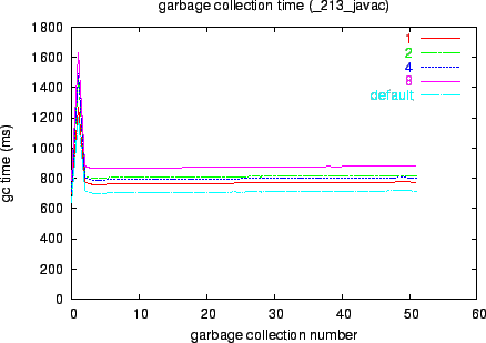
We examine the impact of CTB arrays on the GC.
Since CTB arrays are likely to live for a long time, garbage
collection can be directly affected. Using the _213_javac
benchmark as example with the same experimental setting mentioned
before, GC time was profiled and plotted in Figure 4 for
the default system and configurations with different inlined CTB
sizes. The x-axis is the garbage collection number during the
benchmark run, and the y-axis is the time spent on each collection. We
found that, with these CTB arrays, the GC is slightly slower
than the default system, but not significantly. When inlining more
CTB elements, the GC time is slightly increased. This might be because
the increased size of TIBs exceeds the savings on CTB array
headers when the inlining size gets larger.
We expect a VM with a specific system heap would solve this problem.
The problem mentioned above also poses a challenge for measuring the
overhead of call graph profiling. Furthermore, the call graph profiler
and data structures are written in Java, which implies execution overhead
and memory consumption, affecting
benchmark execution times. To only measure just the overhead of executing
profiling code stubs, we used a compiler option to replace the allocated
caller index by the zero index. When this option is enabled, calls do
not execute the extra load instruction and profiling code stub, but
still allocate CTB arrays for methods. For CFS and SpecJVM98 benchmarks, we
found that usually the first run has some performance degradation
when executing profiling code stubs (up to 9% except for
_201_compress5),
but the degradation is not significant upon reaching a
stable state ( between -2% to 3% ). The performance of SpecJBB2000
is largely unaffected.
Compared to not allocating CTB arrays at all (TIBs, however,
are still expanded), the performance change is also very
small. For our set of benchmarks, it seems that inlining more
CTB array elements does not result in further performance improvements.
| |||||||||||||||||||||||||||||||||||||||||||||||||||||||||||||||||||||||||||||
Table 3 shows the size of the profiled call graph compared to the one constructed by using dynamic CHA. The size of the call graph generated by CHA is shown in the second and third columns where, in the second column, the total number of call edges is followed by those from invokevirtual call sites only. The number of methods is given in the third column. From the second column, we can see that for all benchmarks, the major part of call edges come from invokevirtual instructions. The fourth and fifth columns show the size of profiled call graph and the percentages comparing to the sizes of the CHA call graphs. Call graphs constructed using our profiling code stubs have 20% to 50% fewer call edges than the CHA-based ones. More call edges from invokevirtual sites were reduced than for the other types of call instructions because we took the conservative CHA approach on other types of call instructions to reduce runtime overhead. The reduction for the number of methods is not as significant as for the number of call edges.
Feng Qian 2004-02-16