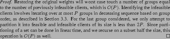
| ||||||||||||||||||||||||||||||||||||||||||||||||||||
|
USENIX '05 Paper
[USENIX '05 Technical Program]
Group Ratio Round-Robin: O(1) Proportional Share
Scheduling
|
|
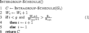
The ![]() intragroup scheduling algorithm
selects a client from the selected group.
All clients within a group have weights
within a factor of two, and
all client weights in a
group
intragroup scheduling algorithm
selects a client from the selected group.
All clients within a group have weights
within a factor of two, and
all client weights in a
group ![]() are normalized with respect to the minimum possible weight,
are normalized with respect to the minimum possible weight,
![]() , for any client in the group.
, for any client in the group.
![]() then
effectively traverses through a group's queue in round-robin order, allocating
each client its normalized weight worth of time quanta.
then
effectively traverses through a group's queue in round-robin order, allocating
each client its normalized weight worth of time quanta.
![]() keeps track of subunitary fractional
time quanta that cannot be used and accumulates them in a deficit value
for each client.
Hence, each client is assigned
either one or two time quanta, based on the client's normalized weight
and its previous allocation.
keeps track of subunitary fractional
time quanta that cannot be used and accumulates them in a deficit value
for each client.
Hence, each client is assigned
either one or two time quanta, based on the client's normalized weight
and its previous allocation.
More specifically, the ![]() intragroup scheduler considers
the scheduling of clients in rounds. A round is one pass through a
group
intragroup scheduler considers
the scheduling of clients in rounds. A round is one pass through a
group ![]() 's run queue of clients from beginning to end. The group run queue
does not need to be sorted in any manner. During each round, the
's run queue of clients from beginning to end. The group run queue
does not need to be sorted in any manner. During each round, the ![]() intragroup algorithm considers the clients in round-robin order and
executes the following simple routine:
intragroup algorithm considers the clients in round-robin order and
executes the following simple routine:
![\begin{codebox}
\Procname{$\procdecl{Intragroup-Schedule}(G)$}
\mi $C \gets G[k]...
...min}^{G}}$
\End
\mi $D_{C} \gets D_{C} - 1$
\mi \Return $C$
\End
\end{codebox}](img70.png)
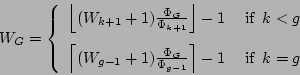
For each runnable client ![]() , the scheduler determines the maximum
number of time quanta that the client can be selected to run in this
round as
, the scheduler determines the maximum
number of time quanta that the client can be selected to run in this
round as
![]() .
.
![]() , the deficit of client
, the deficit of client ![]() after round
after round ![]() , is the time quantum fraction left over after round
, is the time quantum fraction left over after round ![]() :
:
![]() , with
, with
![]() . Thus, in
each round,
. Thus, in
each round, ![]() is allotted one time quantum plus any additional
leftover from the previous round, and
is allotted one time quantum plus any additional
leftover from the previous round, and ![]() keeps track of the
amount of service that
keeps track of the
amount of service that ![]() missed because of rounding down its
allocation to whole time quanta.
We observe that
missed because of rounding down its
allocation to whole time quanta.
We observe that
![]() after
any round
after
any round ![]() so that any client
so that any client ![]() will be allotted one or two
time quanta. Note that if a client is allotted two time quanta, it first executes for one time quantum and then executes for the second
time quantum the next time the intergroup scheduler selects its
respective group again (in general, following a timespan when clients belonging to other groups get to run).
will be allotted one or two
time quanta. Note that if a client is allotted two time quanta, it first executes for one time quantum and then executes for the second
time quantum the next time the intergroup scheduler selects its
respective group again (in general, following a timespan when clients belonging to other groups get to run).
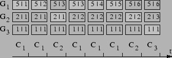
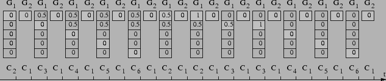
To illustrate how ![]() works with intragroup scheduling,
Figure 2 shows an example
with six clients
works with intragroup scheduling,
Figure 2 shows an example
with six clients ![]() through
through ![]() with weights
12, 3, 3, 2, 2, and 2, respectively.
The six clients will be put in two groups
with weights
12, 3, 3, 2, 2, and 2, respectively.
The six clients will be put in two groups ![]() and
and ![]() with
respective group order 1 and 3 as follows:
with
respective group order 1 and 3 as follows:
![]() and
and ![]() .
The weight
of the groups are
.
The weight
of the groups are
![]() .
. ![]() intergroup scheduling will consider the groups in this order:
intergroup scheduling will consider the groups in this order:
![]() ,
, ![]() ,
, ![]() ,
, ![]() ,
, ![]() ,
, ![]() ,
, ![]() ,
, ![]() ,
, ![]() ,
, ![]() ,
,
![]() ,
, ![]() .
.
![]() will schedule client
will schedule client ![]() every time
every time ![]() is considered for
service since it has only one client.
Since
is considered for
service since it has only one client.
Since
![]() , the normalized weights of clients
, the normalized weights of clients ![]() ,
,
![]() ,
, ![]() ,
, ![]() , and
, and ![]() are 1.5, 1.5, 1, 1, and 1,
respectively. In the
beginning of round 1 in
are 1.5, 1.5, 1, 1, and 1,
respectively. In the
beginning of round 1 in ![]() , each client starts with 0 deficit. As
a result, the intragroup scheduler will run each client in
, each client starts with 0 deficit. As
a result, the intragroup scheduler will run each client in ![]() for
one time quantum during round 1. After the first round, the
deficit for
for
one time quantum during round 1. After the first round, the
deficit for ![]() ,
, ![]() ,
, ![]() ,
, ![]() , and
, and ![]() are 0.5, 0.5, 0, 0, and 0.
In the beginning of round 2, each client gets another
are 0.5, 0.5, 0, 0, and 0.
In the beginning of round 2, each client gets another
![]() allocation, plus any deficit from the first round. As a result, the intragroup
scheduler will select clients
allocation, plus any deficit from the first round. As a result, the intragroup
scheduler will select clients ![]() ,
, ![]() ,
, ![]() ,
, ![]() , and
, and ![]() to run
in order for 2, 2, 1, 1, and 1 time quanta, respectively, during round
2.
The resulting schedule would then be:
to run
in order for 2, 2, 1, 1, and 1 time quanta, respectively, during round
2.
The resulting schedule would then be:
![]() ,
, ![]() ,
, ![]() ,
, ![]() ,
, ![]() ,
, ![]() ,
, ![]() ,
, ![]() ,
, ![]() ,
,
![]() ,
, ![]() ,
, ![]() ,
, ![]() ,
, ![]() ,
, ![]() ,
, ![]() ,
, ![]() ,
, ![]() ,
, ![]() ,
,
![]() ,
, ![]() ,
, ![]() ,
, ![]() ,
, ![]() .
.
|
Runnable clients can be selected for
execution by the scheduler, while clients that are not runnable
cannot.
With no
loss of generality, we assume that a client is created before it can
become runnable, and a client becomes not runnable before it is
terminated. As a result, client creation and termination have no
effect on the ![]() run queues.
run queues.
When a client ![]() with weight
with weight ![]() becomes runnable, it is
inserted into group
becomes runnable, it is
inserted into group ![]() such that
such that ![]() is between
is between
![]() and
and
![]() . If the group was previously
empty, a new group is created, the client becomes the current client of the
group, and
. If the group was previously
empty, a new group is created, the client becomes the current client of the
group, and ![]() , the number of groups, is incremented. If the
group was not previously empty,
, the number of groups, is incremented. If the
group was not previously empty, ![]() inserts the client into the
respective group's run queue right before the current client; it will
be serviced after
all of the other clients in the group have first been considered
for scheduling. The initial deficit
inserts the client into the
respective group's run queue right before the current client; it will
be serviced after
all of the other clients in the group have first been considered
for scheduling. The initial deficit ![]() will be initialized to 0.
will be initialized to 0.
When a newly runnable client ![]() is inserted into its respective
group
is inserted into its respective
group ![]() , the group needs to be moved to its new position on the
ordered group list based on its new group weight. Let this new position be
, the group needs to be moved to its new position on the
ordered group list based on its new group weight. Let this new position be
![]() .
The corresponding
group work and group weight of
.
The corresponding
group work and group weight of ![]() need to be updated and the client's
deficit needs to be initialized. The group weight is simply incremented
by the client's weight. We also want to scale the group work of
need to be updated and the client's
deficit needs to be initialized. The group weight is simply incremented
by the client's weight. We also want to scale the group work of ![]() such
that the work ratio of consecutive groups will continue to be proportional
to their weight ratio:
such
that the work ratio of consecutive groups will continue to be proportional
to their weight ratio:
When a client ![]() with weight
with weight ![]() becomes not runnable, we need
to remove it from the group's run queue. This requires updating the
group's weight, which potentially includes moving the group in the
ordered group list, as well as adjusting the measure of work received
according to the new processor share of the group.
This can be achieved in several ways.
becomes not runnable, we need
to remove it from the group's run queue. This requires updating the
group's weight, which potentially includes moving the group in the
ordered group list, as well as adjusting the measure of work received
according to the new processor share of the group.
This can be achieved in several ways. ![]() is optimized to
efficiently deal with the common situation when a blocked client may
rapidly switch back to the runnable state again. This approach is
based on ``lazy'' removal, which minimizes overhead associated
with adding and removing a client, while at the same time preserving
the service rights and service order of the runnable clients. Since a
client blocks when it is running, we know that it will take another
full intragroup round before the client will be considered again. The only action
when a client blocks is to set a flag on the client, marking it for
removal. If the client becomes runnable by the next time it is
selected, we reset the flag and run the client as
usual. Otherwise, we remove the client from
is optimized to
efficiently deal with the common situation when a blocked client may
rapidly switch back to the runnable state again. This approach is
based on ``lazy'' removal, which minimizes overhead associated
with adding and removing a client, while at the same time preserving
the service rights and service order of the runnable clients. Since a
client blocks when it is running, we know that it will take another
full intragroup round before the client will be considered again. The only action
when a client blocks is to set a flag on the client, marking it for
removal. If the client becomes runnable by the next time it is
selected, we reset the flag and run the client as
usual. Otherwise, we remove the client from ![]() . In the latter
situation, as in the case of client arrivals, the group may need to be
moved to a new position on the ordered group list based on its new
group weight. The corresponding group weight is updated by
subtracting the client's weight from the group weight. The
corresponding group work is scaled by the same rules as for client
insertion, depending on the new position of the group and its next neighbor.
After performing these removal operations,
. In the latter
situation, as in the case of client arrivals, the group may need to be
moved to a new position on the ordered group list based on its new
group weight. The corresponding group weight is updated by
subtracting the client's weight from the group weight. The
corresponding group work is scaled by the same rules as for client
insertion, depending on the new position of the group and its next neighbor.
After performing these removal operations, ![]() resumes scheduling
from the largest weight group in the system.
resumes scheduling
from the largest weight group in the system.
Whenever a client ![]() blocks during round
blocks during round ![]() , we set
, we set
![]() ,
where
,
where ![]() is the service that the client received during round
is the service that the client received during round
![]() until it blocked. This preserves the client's credit in case it
returns by the next round, while also limiting the deficit to
until it blocked. This preserves the client's credit in case it
returns by the next round, while also limiting the deficit to ![]() so
that a client cannot gain credit by blocking.
However,
the group consumes
so
that a client cannot gain credit by blocking.
However,
the group consumes ![]() tu (its work is incremented) no matter how long
the client runs. Therefore, the client forfeits its extra credit
whenever it is unable to consume its allocation.
tu (its work is incremented) no matter how long
the client runs. Therefore, the client forfeits its extra credit
whenever it is unable to consume its allocation.
If the client fails to return by the next round, we may remove it. Having kept the weight of the group to the old value for an extra round has no adverse effects on fairness, despite the slight increase in service seen by the group during the last round. By scaling the work of the group and rounding up, we determine its future allocation and thus make sure the group will not have received undue service. We also immediately resume the scheduler from the first (largest) group in the readjusted group list, so that any minor discrepancies caused by rounding may be smoothed out by a first pass through the group list.
We now present extensions to ![]() for scheduling a
for scheduling a ![]() -way
multiprocessor system from a single, centralized queue. This simple
scheme, which we refer to as
-way
multiprocessor system from a single, centralized queue. This simple
scheme, which we refer to as ![]() , preserves the good
fairness and time complexity properties of
, preserves the good
fairness and time complexity properties of ![]() in small-scale
multiprocessor systems, which are increasingly common today, even in
the form of multi-core processors. We first describe the basic
in small-scale
multiprocessor systems, which are increasingly common today, even in
the form of multi-core processors. We first describe the basic ![]() scheduling algorithm, then discuss dynamic considerations. Table
2 lists terminology we use. To deal with the
problem of infeasible client weights, we then show how
scheduling algorithm, then discuss dynamic considerations. Table
2 lists terminology we use. To deal with the
problem of infeasible client weights, we then show how ![]() uses its
grouping strategy in a novel weight readjustment algorithm.
uses its
grouping strategy in a novel weight readjustment algorithm.
To handle this situation while maintaining fairness, ![]() introduces the notion of a frontlog. The frontlog
introduces the notion of a frontlog. The frontlog ![]() for
some client
for
some client ![]() running on a processor
running on a processor ![]() (
(![]() ) is
defined as the number of time quanta for
) is
defined as the number of time quanta for ![]() accumulated as
accumulated as ![]() gets selected by
gets selected by ![]() and cannot run because it is already running
on
and cannot run because it is already running
on ![]() . The frontlog
. The frontlog ![]() is then queued up on
is then queued up on ![]() .
.
Given a client that would be scheduled by ![]() but is already
running on another processor,
but is already
running on another processor, ![]() uses the frontlog to assign
the client a time quantum now but defer the client's use of it until
later. Whenever a processor finishes running a client for a time
quantum,
uses the frontlog to assign
the client a time quantum now but defer the client's use of it until
later. Whenever a processor finishes running a client for a time
quantum, ![]() checks whether the client has a non-zero frontlog,
and, if so, continues running the client for another time quantum and
decrements its frontlog by one, without consulting the central queue. The frontlog mechanism not only
ensures that a client receives its proportional share allocation, it
also takes advantage of any cache affinity by continuing to run the
client on the same processor.
checks whether the client has a non-zero frontlog,
and, if so, continues running the client for another time quantum and
decrements its frontlog by one, without consulting the central queue. The frontlog mechanism not only
ensures that a client receives its proportional share allocation, it
also takes advantage of any cache affinity by continuing to run the
client on the same processor.
When a processor finishes running a client for a time quantum and its
frontlog is zero, we call the processor idle. ![]() schedules a client to run on the idle processor by performing
a
schedules a client to run on the idle processor by performing
a ![]() scheduling decision on the central queue. If the selected
client is already running on some other processor, we increase its
frontlog and repeat the
scheduling decision on the central queue. If the selected
client is already running on some other processor, we increase its
frontlog and repeat the ![]() scheduling, each time incrementing the
frontlog of the selected client, until we find a client that is not
currently running. We assign this client to the idle processor for one
time quantum. This description assumes that there are least
scheduling, each time incrementing the
frontlog of the selected client, until we find a client that is not
currently running. We assign this client to the idle processor for one
time quantum. This description assumes that there are least ![]() clients in the system. Otherwise, scheduling is easy: an idle processor will either run the client it just ran, or idles until more clients arrive. In effect,
each client will simply be assigned its own processor.
Whenever a processor needs to perform a scheduling decision, it thus
executes the following routine:
clients in the system. Otherwise, scheduling is easy: an idle processor will either run the client it just ran, or idles until more clients arrive. In effect,
each client will simply be assigned its own processor.
Whenever a processor needs to perform a scheduling decision, it thus
executes the following routine:
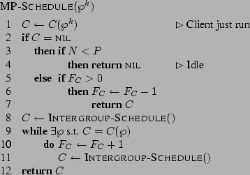
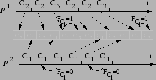
To illustrate ![]() scheduling, Figure 3 shows
an example on a dual-processor system with three clients
scheduling, Figure 3 shows
an example on a dual-processor system with three clients ![]() ,
, ![]() ,
and
,
and ![]() of weights 3, 2, and 1, respectively.
of weights 3, 2, and 1, respectively. ![]() and
and ![]() will
then be part of the order 1 group (assume
will
then be part of the order 1 group (assume ![]() is before
is before ![]() in the
round-robin queue of this group), whereas
in the
round-robin queue of this group), whereas ![]() is part of the order 0
group. The
is part of the order 0
group. The ![]() schedule is
schedule is ![]() ,
, ![]() ,
, ![]() ,
, ![]() ,
, ![]() ,
,
![]() .
. ![]() will then select
will then select ![]() to run, and
to run, and ![]() selects
selects
![]() . When
. When ![]() finishes, according to
finishes, according to ![]() , it will select
, it will select
![]() once more, whereas
once more, whereas ![]() selects
selects ![]() again. When
again. When ![]() again selects the next
again selects the next ![]() client, which is
client, which is ![]() , it finds that it
is already running on
, it finds that it
is already running on ![]() and thus we set
and thus we set ![]() and select
the next client, which is
and select
the next client, which is ![]() , to run on
, to run on ![]() . When
. When ![]() finishes running
finishes running ![]() for its second time quantum, it finds
for its second time quantum, it finds ![]() , sets
, sets ![]() and continues running
and continues running ![]() without any
scheduling decision on the
without any
scheduling decision on the ![]() queue.
queue.
|
![]() provides fair and responsive allocations by creating
frontlogs for newly arriving clients. Each new client is assigned a
frontlog equal to a fraction of the total current frontlog in the
system based on its proportional share. Each processor now maintains
a queue of frontlog clients and a new client with a frontlog is
immediately assigned to one of the processor frontlog queues. Rather
than running its currently running client until it completes its
frontlog, each processor now round robins among clients in its
frontlog queue. Given that frontlogs are small in practice,
round-robin scheduling is used for frontlog clients for its simplicity
and fairness.
provides fair and responsive allocations by creating
frontlogs for newly arriving clients. Each new client is assigned a
frontlog equal to a fraction of the total current frontlog in the
system based on its proportional share. Each processor now maintains
a queue of frontlog clients and a new client with a frontlog is
immediately assigned to one of the processor frontlog queues. Rather
than running its currently running client until it completes its
frontlog, each processor now round robins among clients in its
frontlog queue. Given that frontlogs are small in practice,
round-robin scheduling is used for frontlog clients for its simplicity
and fairness. ![]() balances the frontlog load on the processors
by placing new frontlog clients on the processor with the smallest
frontlog summed across all its frontlog clients.
balances the frontlog load on the processors
by placing new frontlog clients on the processor with the smallest
frontlog summed across all its frontlog clients.
More precisely, whenever a client ![]() arrives, and it belongs in
group
arrives, and it belongs in
group ![]() ,
, ![]() performs the same group operations as in the
single processor
performs the same group operations as in the
single processor ![]() algorithm.
algorithm. ![]() finds the processor
finds the processor
![]() with the smallest frontlog, then creates a frontlog for client
with the smallest frontlog, then creates a frontlog for client
![]() on
on ![]() of length
of length
![]() , where
, where
![]() is the total frontlog on all the processors. Let
is the total frontlog on all the processors. Let ![]() . Then, assuming no further clients arrive,
. Then, assuming no further clients arrive, ![]() will
round-robin between
will
round-robin between ![]() and
and ![]() and run
and run ![]() for
for ![]() and
and ![]() for
for ![]() time quanta.
time quanta.
When a client becomes not runnable, ![]() uses the same lazy
removal mechanism used in
uses the same lazy
removal mechanism used in ![]() . If it is removed from the run queue
and has a frontlog,
. If it is removed from the run queue
and has a frontlog, ![]() simply discards it since each client is
assigned a frontlog based on the current state of the system when it
becomes runnable again.
simply discards it since each client is
assigned a frontlog based on the current state of the system when it
becomes runnable again.
To understand the problem of weight readjustment,
consider the sequence of all clients, ordered by weight:
![]() with
with
![]() .
We call the subsequence
.
We call the subsequence
![]()
![]() -feasible, if
-feasible, if
![]() .
.
The feasibility problem is then to identify the least ![]() (denoted the
feasibility threshold,
(denoted the
feasibility threshold, ![]() ) such that
) such that ![]() is
is ![]() -feasible. If
-feasible. If ![]() , then the client mix is feasible. Otherwise,
the infeasible set
, then the client mix is feasible. Otherwise,
the infeasible set
![]() contains
the infeasible clients, whose weight needs to be scaled down to
contains
the infeasible clients, whose weight needs to be scaled down to ![]() of the resulting total weight.
The cardinality
of the resulting total weight.
The cardinality ![]() of the infeasible set is less than
of the infeasible set is less than ![]() . However, the sorted sequence
. However, the sorted sequence ![]() is expensive to maintain, such that traversing it and identifying the feasibility threshold is not an efficient solution.
is expensive to maintain, such that traversing it and identifying the feasibility threshold is not an efficient solution.
![]() leverages its grouping strategy to perform fast weight
readjustment.
leverages its grouping strategy to perform fast weight
readjustment. ![]() starts with the unmodified client
weights, finds the set
starts with the unmodified client
weights, finds the set ![]() of infeasible clients, and adjust their weights to be feasible. To construct
of infeasible clients, and adjust their weights to be feasible. To construct ![]() , the algorithm traverses the list of groups in decreasing order of their group order
, the algorithm traverses the list of groups in decreasing order of their group order ![]() , until it finds a group not all of whose clients are infeasible.
We denote by
, until it finds a group not all of whose clients are infeasible.
We denote by ![]() the cardinality of
the cardinality of ![]() and by
and by ![]() the sum of
weights of the clients in
the sum of
weights of the clients in ![]() ,
,
![]() .
The
.
The ![]() weight readjustment algorithm is as follows:
weight readjustment algorithm is as follows:
The correctness of the algorithm is based on Lemma 2. Let some group ![]() span the subsequence
span the subsequence ![]() of the sequence of ordered clients
of the sequence of ordered clients ![]() . Then
. Then
![]() and it is easy to show:
and it is easy to show:
![]() can alternatively use a more complicated but lower time
complexity divide-and-conquer algorithm to find the infeasible clients
in
can alternatively use a more complicated but lower time
complexity divide-and-conquer algorithm to find the infeasible clients
in ![]() . In this case,
. In this case, ![]() partitions
partitions ![]() around its median
around its median ![]() into
into ![]() , the set of
, the set of ![]() clients that have weight less than
clients that have weight less than
![]() and
and ![]() , the set of
, the set of ![]() clients that have weight larger than
clients that have weight larger than
![]() . By Lemma 2, if
. By Lemma 2, if ![]() is feasible,
is feasible,
![]() is feasible, and we recurse on
is feasible, and we recurse on ![]() . Otherwise,
all clients in
. Otherwise,
all clients in
![]() are infeasible, and we
recurse on
are infeasible, and we
recurse on ![]() to find all infeasible clients.
The algorithm finishes when the set we need to recurse on is
empty:
to find all infeasible clients.
The algorithm finishes when the set we need to recurse on is
empty:
Once all infeasible clients have been identified,
![]() determines
the sum of the weights of all feasible clients,
determines
the sum of the weights of all feasible clients,
![]() . We can now compute the new total weight in the system as
. We can now compute the new total weight in the system as
![]() , namely the solution to the
equation
, namely the solution to the
equation
![]() . Once we have the adjusted
. Once we have the adjusted
![]() , we change all the weights for the infeasible clients in
, we change all the weights for the infeasible clients in ![]() to
to
![]() .
Lemma 6 in Section
4.2 shows the readjustment algorithm runs in
time
.
Lemma 6 in Section
4.2 shows the readjustment algorithm runs in
time ![]() and is thus asymptotically optimal, since there can be
and is thus asymptotically optimal, since there can be
![]() infeasible clients.
infeasible clients.
We analyze the fairness and complexity of ![]() and
and ![]() . To
analyze fairness, we use a more formal notion of proportional fairness
defined as service error, a measure widely used
[1,7,9,17,18,19,25,27]
in the analysis of scheduling algorithms. To simplify the analysis,
we will assume that clients are always runnable and derive fairness
bounds for such a case. Subsequently, we address the impact of
arrivals and departures.
. To
analyze fairness, we use a more formal notion of proportional fairness
defined as service error, a measure widely used
[1,7,9,17,18,19,25,27]
in the analysis of scheduling algorithms. To simplify the analysis,
we will assume that clients are always runnable and derive fairness
bounds for such a case. Subsequently, we address the impact of
arrivals and departures.
We use a strict measure of
service error (equivalent in this context to the Normalized Worst-case Fair Index [1]) relative to Generalized Processor Sharing
(GPS) [16], an idealized model that
achieves perfect fairness:
![]() , an
ideal state in which each client
, an
ideal state in which each client ![]() always receives service exactly
proportional to its weight. Although all real-world schedulers
must time-multiplex resources in time units of finite size
and thus cannot maintain perfect fairness, some algorithms stay closer
to perfect fairness than others and therefore have less service error.
We quantify how close an algorithm gets to perfect fairness using
the client service time error, which is the difference
between the service received by client
always receives service exactly
proportional to its weight. Although all real-world schedulers
must time-multiplex resources in time units of finite size
and thus cannot maintain perfect fairness, some algorithms stay closer
to perfect fairness than others and therefore have less service error.
We quantify how close an algorithm gets to perfect fairness using
the client service time error, which is the difference
between the service received by client ![]() and its share of the total
work done by the processor:
and its share of the total
work done by the processor:
![]() .
A positive service time error indicates that a client has
received more than its ideal share over a time interval; a negative
error indicates that it has received less. To be precise, the error
.
A positive service time error indicates that a client has
received more than its ideal share over a time interval; a negative
error indicates that it has received less. To be precise, the error
![]() measures how much time a client
measures how much time a client ![]() has received beyond
its ideal allocation. A proportional share scheduler should
minimize the absolute value of the allocation error
of all clients with minimal scheduling overhead.
has received beyond
its ideal allocation. A proportional share scheduler should
minimize the absolute value of the allocation error
of all clients with minimal scheduling overhead.
We provide bounds on the service error of ![]() and
and ![]() .
To do this, we define two other measures of
service error. The group service time error is a similar
measure for groups that quantifies the fairness of allocating the
processor among groups:
.
To do this, we define two other measures of
service error. The group service time error is a similar
measure for groups that quantifies the fairness of allocating the
processor among groups:
![]() .
The group-relative service time error represents the service time
error of client
.
The group-relative service time error represents the service time
error of client ![]() if there were only a single group
if there were only a single group ![]() in the
scheduler and is a measure of the service error of a client with
respect to the work done on behalf of its group:
in the
scheduler and is a measure of the service error of a client with
respect to the work done on behalf of its group:
![]() . We first show bounds on the group
service error of the intergroup scheduling algorithm. We then show
bounds on the group-relative service error of the intragroup
scheduling algorithm. We combine these results to obtain the overall
client service error bounds. We also discuss the scheduling
overhead of
. We first show bounds on the group
service error of the intergroup scheduling algorithm. We then show
bounds on the group-relative service error of the intragroup
scheduling algorithm. We combine these results to obtain the overall
client service error bounds. We also discuss the scheduling
overhead of ![]() and
and ![]() in terms of their
time complexity. We show that both algorithms can make scheduling
decisions in
in terms of their
time complexity. We show that both algorithms can make scheduling
decisions in ![]() time with
time with ![]() service error given a constant
number of groups. Due to space constraints, most of the proofs are
omitted. Further proof details are available in [5].
service error given a constant
number of groups. Due to space constraints, most of the proofs are
omitted. Further proof details are available in [5].
For the case when the weight ratios of consecutive groups in the group list are integers, we get the following:
Proof sketch: If the group currently scheduled isIn the general case, we get similar, but slightly weaker bounds.
The proof for this case (omitted) follows reasoning similar to that of the previous lemma, but with several additional complications.
It is clear that the lower bound is minimized when setting ![]() . Thus,
we have
. Thus,
we have
Based on the identity
![]() which holds for any group
which holds for any group ![]() and any client
and any client ![]() , we can combine the inter- and intragroup analyses to bound the overall
fairness of
, we can combine the inter- and intragroup analyses to bound the overall
fairness of ![]() .
.
The negative error of ![]() is thus bounded by
is thus bounded by
![]() and the positive error by
and the positive error by ![]() . Recall,
. Recall, ![]() , the number
of groups, does not depend on the number of clients in the system.
, the number
of groups, does not depend on the number of clients in the system.
![]() manages to bound its service error by
manages to bound its service error by ![]() while
maintaining a strict
while
maintaining a strict ![]() scheduling overhead.
The intergroup scheduler either selects the next group
in the list, or reverts to the first one, which takes constant
time. The intragroup scheduler is even simpler, as it just picks the
next client to run from the unordered round robin list of the
group. Adding and removing a client is worst-case
scheduling overhead.
The intergroup scheduler either selects the next group
in the list, or reverts to the first one, which takes constant
time. The intragroup scheduler is even simpler, as it just picks the
next client to run from the unordered round robin list of the
group. Adding and removing a client is worst-case ![]() when a group
needs to be relocated in the ordered list of groups. This could of
course be done in
when a group
needs to be relocated in the ordered list of groups. This could of
course be done in ![]() time (using binary search, for example), but the small value of
time (using binary search, for example), but the small value of ![]() in practice
does not justify a more complicated algorithm.
in practice
does not justify a more complicated algorithm.
The space complexity of ![]() is
is
![]() . The
only additional data structure beyond the unordered lists of clients
is an ordered list of length
. The
only additional data structure beyond the unordered lists of clients
is an ordered list of length ![]() to organize the groups.
to organize the groups.
The frontlogs create an additional complication when analyzing the
time complexity of ![]() . When an idle processor looks for its
next client, it runs the simple
. When an idle processor looks for its
next client, it runs the simple ![]()
![]() algorithm to find a client
algorithm to find a client
![]() . If
. If ![]() is not running on any other processor, we are done,
but otherwise we place it on the frontlog
and then we must rerun the
is not running on any other processor, we are done,
but otherwise we place it on the frontlog
and then we must rerun the ![]() algorithm until we find a client that is not running on any other
processor. Since for each such client, we increase its
allocation on the processor it runs, the amortized time complexity
remains
algorithm until we find a client that is not running on any other
processor. Since for each such client, we increase its
allocation on the processor it runs, the amortized time complexity
remains ![]() . The upper bound on the time that any single
scheduling decision takes is given by the maximum length
of any scheduling sequence of
. The upper bound on the time that any single
scheduling decision takes is given by the maximum length
of any scheduling sequence of ![]() consisting of only
some fixed subset of
consisting of only
some fixed subset of ![]() clients.
clients.
Thus, the length of any schedule consisting of at most ![]() clients is
clients is ![]() .
Even when a processor has frontlogs for several clients queued up on it, it will schedule in
.
Even when a processor has frontlogs for several clients queued up on it, it will schedule in ![]() time, since it performs round-robin among the frontlogged clients.
Client arrivals and departures take
time, since it performs round-robin among the frontlogged clients.
Client arrivals and departures take ![]() time because of the need to
readjust group weights in the saved list of groups. Moreover, if we
also need to use the weight readjustment algorithm, we incur an
additional
time because of the need to
readjust group weights in the saved list of groups. Moreover, if we
also need to use the weight readjustment algorithm, we incur an
additional ![]() overhead on client arrivals and departures.
overhead on client arrivals and departures.
For small ![]() , the
, the ![]() sorting approach to
determine infeasible clients in the last group considered is simpler
and in practice performs better than the
sorting approach to
determine infeasible clients in the last group considered is simpler
and in practice performs better than the ![]() recursive partitioning.
Finally, altering the active group
structure to reflect the new weights is a
recursive partitioning.
Finally, altering the active group
structure to reflect the new weights is a ![]() operation, as two groups may need to be re-inserted in the ordered list
of groups.
operation, as two groups may need to be re-inserted in the ordered list
of groups.
Section 5.1 presents
simulation results comparing the proportional sharing
accuracy of ![]() and
and ![]() against WRR, WFQ [18], SFQ [13],
VTRR [17], and SRR [9].
The simulator enabled us to isolate the impact of the scheduling
algorithms themselves and examine the scheduling behavior of these
different algorithms across hundreds of thousands of different
combinations of clients with different weight values.
against WRR, WFQ [18], SFQ [13],
VTRR [17], and SRR [9].
The simulator enabled us to isolate the impact of the scheduling
algorithms themselves and examine the scheduling behavior of these
different algorithms across hundreds of thousands of different
combinations of clients with different weight values.
Section 5.2 presents detailed measurements of real
kernel scheduler performance by comparing our prototype ![]() Linux
implementation against the standard Linux scheduler, a WFQ scheduler,
and a VTRR scheduler.
The experiments we have done quantify the scheduling overhead and
proportional share allocation accuracy of these schedulers in a real
operating system environment under a number of different workloads.
Linux
implementation against the standard Linux scheduler, a WFQ scheduler,
and a VTRR scheduler.
The experiments we have done quantify the scheduling overhead and
proportional share allocation accuracy of these schedulers in a real
operating system environment under a number of different workloads.
All our kernel scheduler measurements were performed on an IBM Netfinity 4500 system with one or two 933 MHz Intel Pentium III CPUs, 512 MB RAM, and 9 GB hard drive. The system was installed with the Debian GNU/Linux distribution version 3.0 and all schedulers were implemented using Linux kernel version 2.4.19. The measurements were done by using a minimally intrusive tracing facility that writes timestamped event identifiers into a memory log and takes advantage of the high-resolution clock cycle counter available with the Intel CPU, providing measurement resolution at the granularity of a few nanoseconds. Getting a timestamp simply involved reading the hardware cycle counter register. We measured the timestamp overhead to be roughly 35 ns per event.
The kernel scheduler measurements were performed on a fully functional system. All experiments were performed with all system functions running and the system connected to the network. At the same time, an effort was made to eliminate variations in the test environment to make the experiments repeatable.
|
|
|
|
||||
|
|
|
|
We built a scheduling simulator that measures the service time error,
described in Section 4, of a scheduler on a set
of clients. The simulator takes four inputs, the scheduling
algorithm, the number of clients ![]() , the total sum of weights
, the total sum of weights ![]() ,
and the number of client-weight combinations. The simulator
randomly assigns weights to clients and scales the weights to ensure that
they add up to
,
and the number of client-weight combinations. The simulator
randomly assigns weights to clients and scales the weights to ensure that
they add up to ![]() . It then schedules the clients using the specified
algorithm as a real scheduler would, assuming no client blocks, and tracks the resulting service
time error. The simulator runs the scheduler until the resulting
schedule repeats, then computes the maximum (most positive) and
minimum (most negative) service time error across the nonrepeating
portion of the schedule for the given set of clients and weight
assignments. This process is repeated for the specified number of
client-weight combinations. We then compute the maximum service time
error and minimum service time error for the specified number of
client-weight combinations to obtain a ``worst-case'' error range.
. It then schedules the clients using the specified
algorithm as a real scheduler would, assuming no client blocks, and tracks the resulting service
time error. The simulator runs the scheduler until the resulting
schedule repeats, then computes the maximum (most positive) and
minimum (most negative) service time error across the nonrepeating
portion of the schedule for the given set of clients and weight
assignments. This process is repeated for the specified number of
client-weight combinations. We then compute the maximum service time
error and minimum service time error for the specified number of
client-weight combinations to obtain a ``worst-case'' error range.
To measure proportional fairness accuracy, we ran simulations for each
scheduling algorithm on 45 different combinations of ![]() and
and ![]() (32 up
to 8192 clients and 16384 up to 262144 total weight, respectively). Since the proportional sharing accuracy of a
scheduler is often most clearly illustrated with skewed weight
distributions, one of the clients was given a weight equal to 10
percent of
(32 up
to 8192 clients and 16384 up to 262144 total weight, respectively). Since the proportional sharing accuracy of a
scheduler is often most clearly illustrated with skewed weight
distributions, one of the clients was given a weight equal to 10
percent of ![]() . All of the other clients were then randomly assigned
weights to sum to the remaining 90 percent of
. All of the other clients were then randomly assigned
weights to sum to the remaining 90 percent of ![]() . For each pair
. For each pair
![]() , we ran 2500 client-weight combinations and determined the
resulting worst-case error range.
, we ran 2500 client-weight combinations and determined the
resulting worst-case error range.
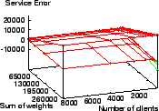
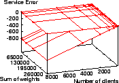
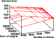
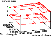
The worst-case service time error ranges for WRR, WFQ, SFQ, VTRR, SRR,
and ![]() with these skewed weight distributions are in
Figures 4 to 9.
Due to space constraints, WF
with these skewed weight distributions are in
Figures 4 to 9.
Due to space constraints, WF![]() Q error is not shown since the results
simply verify its known mathematical error bounds of
Q error is not shown since the results
simply verify its known mathematical error bounds of ![]() and
and ![]() tu.
Each figure consists of a graph of the error range for the respective
scheduling algorithm. Each graph shows two surfaces representing the
maximum and minimum service time error as a function of
tu.
Each figure consists of a graph of the error range for the respective
scheduling algorithm. Each graph shows two surfaces representing the
maximum and minimum service time error as a function of ![]() and
and ![]() for the same range of values of
for the same range of values of ![]() and
and ![]() .
Figure 4 shows WRR's service time error is between
.
Figure 4 shows WRR's service time error is between
![]() tu and
tu and ![]() tu.
Figure 5 shows WFQ's service time error is between
tu.
Figure 5 shows WFQ's service time error is between
![]() tu and
tu and ![]() tu, which is much less than WRR.
Figure 6 shows SFQ's service time error is between
tu, which is much less than WRR.
Figure 6 shows SFQ's service time error is between
![]() tu and
tu and ![]() tu, which is almost a mirror image of WFQ.
Figure 7 shows VTRR's service error is between
tu, which is almost a mirror image of WFQ.
Figure 7 shows VTRR's service error is between
![]() tu and
tu and ![]() tu.
Figure 8 shows SRR's service error is between
tu.
Figure 8 shows SRR's service error is between
![]() tu and
tu and ![]() tu.
tu.
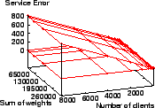
In comparison, Figure 9 shows the service time error
for ![]() only ranges from
only ranges from ![]() to
to ![]() tu.
tu. ![]() has a smaller
error range than all of the other schedulers measured except WF
has a smaller
error range than all of the other schedulers measured except WF![]() Q.
Q.
![]() has both a smaller negative and smaller positive service time
error than WRR, VTRR, and SRR. While
has both a smaller negative and smaller positive service time
error than WRR, VTRR, and SRR. While ![]() has a much smaller
positive service error than WFQ, WFQ does have a smaller negative
service time error since it is bounded below at
has a much smaller
positive service error than WFQ, WFQ does have a smaller negative
service time error since it is bounded below at ![]() . Similarly,
. Similarly,
![]() has a much smaller negative service error than SFQ, though
SFQ's positive error is less since it is bounded above at
has a much smaller negative service error than SFQ, though
SFQ's positive error is less since it is bounded above at ![]() .
Considering the total service error range of each scheduler,
.
Considering the total service error range of each scheduler, ![]() provides well over two orders of magnitude better proportional sharing
accuracy than WRR, WFQ, SFQ, VTRR, and SRR. Unlike the other
schedulers, these results show that
provides well over two orders of magnitude better proportional sharing
accuracy than WRR, WFQ, SFQ, VTRR, and SRR. Unlike the other
schedulers, these results show that ![]() combines the benefits of
low service time errors with its ability to schedule in
combines the benefits of
low service time errors with its ability to schedule in ![]() time.
time.
Note that as the weight skew becomes more accentuated, the service error
can grow dramatically. Thus, increasing the skew from 10 to 50 percent
results in more than a fivefold increase in the error magnitude for
SRR, WFQ, and SFQ, and also significantly worse errors for WRR and
VTRR. In contrast, the error of ![]() is still bounded by small
constants:
is still bounded by small
constants: ![]() and
and ![]() .
.
We also measured the service error of ![]() using this simulator
configured for an 8 processor system, where the weight distribution
was the same as for the uniprocessor simulations above. Note that the
client given 0.1 of the total weight was feasible, since
using this simulator
configured for an 8 processor system, where the weight distribution
was the same as for the uniprocessor simulations above. Note that the
client given 0.1 of the total weight was feasible, since
![]() .
Figure 10 shows
.
Figure 10 shows ![]() 's service error is between
's service error is between
![]() tu and
tu and ![]() tu, slightly better than for the uniprocessor case,
a benefit of being able to run multiple clients in parallel.
Figure 11 shows the maximum number of scheduling
decisions that an idle processor needs to perform until it finds a
client that is not running. This did not exceed seven, indicating
that the number of decisions needed in practice is well below the
worst-case bounds shown in Theorem 3.
tu, slightly better than for the uniprocessor case,
a benefit of being able to run multiple clients in parallel.
Figure 11 shows the maximum number of scheduling
decisions that an idle processor needs to perform until it finds a
client that is not running. This did not exceed seven, indicating
that the number of decisions needed in practice is well below the
worst-case bounds shown in Theorem 3.
Figure 12 shows the average execution time required
by each scheduler to select a client to execute. Results for ![]() ,
VTRR, WFQ, and Linux were obtained on uniprocessor system, and
results for
,
VTRR, WFQ, and Linux were obtained on uniprocessor system, and
results for ![]() and LinuxMP were obtained running on a
dual-processor system. Dual-processor results for WFQ and VTRR are
not shown since MP-ready implementations of them were not available.
and LinuxMP were obtained running on a
dual-processor system. Dual-processor results for WFQ and VTRR are
not shown since MP-ready implementations of them were not available.
For this experiment,
the particular implementation details of the WFQ scheduler affect the
overhead, so we include results from two different implementations of
WFQ. In the first, labeled ``WFQ [![]() ]'', the run queue is
implemented as a simple linked list which must be searched on every
scheduling decision. The second, labeled ``WFQ [
]'', the run queue is
implemented as a simple linked list which must be searched on every
scheduling decision. The second, labeled ``WFQ [![]() ]'', uses a
heap-based priority queue with
]'', uses a
heap-based priority queue with ![]() insertion time. To
maintain the heap-based priority queue, we used a
fixed-length array. If the number of clients ever exceeds the length
of the array, a costly array reallocation must be performed. Our
initial array size was large enough to contain more than 400 clients,
so this additional cost is not reflected in our measurements.
insertion time. To
maintain the heap-based priority queue, we used a
fixed-length array. If the number of clients ever exceeds the length
of the array, a costly array reallocation must be performed. Our
initial array size was large enough to contain more than 400 clients,
so this additional cost is not reflected in our measurements.
As shown in Figure 12, the increase in scheduling
overhead as the number of clients increases varies a great deal
between different schedulers. ![]() has the smallest scheduling
overhead. It requires roughly 300 ns to select a client to execute
and the scheduling overhead is essentially constant for all numbers of
clients. While VTRR scheduling overhead is also constant,
has the smallest scheduling
overhead. It requires roughly 300 ns to select a client to execute
and the scheduling overhead is essentially constant for all numbers of
clients. While VTRR scheduling overhead is also constant, ![]() has
less overhead because its computations are simpler to perform than the
virtual time calculations required by VTRR. In contrast, the overhead
for Linux and for
has
less overhead because its computations are simpler to perform than the
virtual time calculations required by VTRR. In contrast, the overhead
for Linux and for ![]() WFQ scheduling grows linearly with the number
of clients. Both of these schedulers impose more than 200 times more
overhead than
WFQ scheduling grows linearly with the number
of clients. Both of these schedulers impose more than 200 times more
overhead than ![]() when scheduling a mix of 400 clients.
when scheduling a mix of 400 clients.
![]() WFQ has much smaller overhead than Linux or
WFQ has much smaller overhead than Linux or ![]() WFQ, but it still imposes significantly more overhead than
WFQ, but it still imposes significantly more overhead than ![]() ,
with 8 times more overhead than
,
with 8 times more overhead than ![]() when scheduling a mix of
400 clients.
Figure 12 also shows that
when scheduling a mix of
400 clients.
Figure 12 also shows that ![]() provides the same
provides the same
![]() scheduling overhead on a multiprocessor, although the absolute
time to schedule is somewhat higher due to additional costs associated
with scheduling in multiprocessor systems. The results show that
scheduling overhead on a multiprocessor, although the absolute
time to schedule is somewhat higher due to additional costs associated
with scheduling in multiprocessor systems. The results show that
![]() provides substantially lower overhead than the standard Linux
scheduler, which suffers from complexity that grows linearly with the
number of clients.
Because of the importance of constant scheduling overhead in server
systems, Linux has switched to Ingo Molnar's
provides substantially lower overhead than the standard Linux
scheduler, which suffers from complexity that grows linearly with the
number of clients.
Because of the importance of constant scheduling overhead in server
systems, Linux has switched to Ingo Molnar's ![]() scheduler in the
Linux 2.6 kernel. As a comparison, we also repeated this
microbenchmark experiment with that scheduler and found that
scheduler in the
Linux 2.6 kernel. As a comparison, we also repeated this
microbenchmark experiment with that scheduler and found that ![]() still runs over 30 percent faster.
still runs over 30 percent faster.
As another experiment, we measured the scheduling overhead of the
various schedulers for ![]() [21], a benchmark
used in the Linux community for measuring scheduler performance with
large numbers of processes entering and leaving the run queue at all
times. It creates groups of readers and writers, each group having 20
reader tasks and 20 writer tasks, and each writer writes 100 small
messages to each of the other 20 readers. This is a total of 2000
messages sent per writer, per group, or 40000 messages per group.
We ran a modified version of hackbench to give each reader and each
writer a random weight between 1 and 40. We performed these tests on
the same set of schedulers for 1 group up to 100 groups. Using 100
groups results in up to 8000 processes running. Because hackbench
frequently inserts and removes clients from the run queue, the cost of
client insertion and removal is a more significant factor for this
benchmark. The results show that the simple dynamic group adjustments
described in Section 2.3 have low overhead, since
[21], a benchmark
used in the Linux community for measuring scheduler performance with
large numbers of processes entering and leaving the run queue at all
times. It creates groups of readers and writers, each group having 20
reader tasks and 20 writer tasks, and each writer writes 100 small
messages to each of the other 20 readers. This is a total of 2000
messages sent per writer, per group, or 40000 messages per group.
We ran a modified version of hackbench to give each reader and each
writer a random weight between 1 and 40. We performed these tests on
the same set of schedulers for 1 group up to 100 groups. Using 100
groups results in up to 8000 processes running. Because hackbench
frequently inserts and removes clients from the run queue, the cost of
client insertion and removal is a more significant factor for this
benchmark. The results show that the simple dynamic group adjustments
described in Section 2.3 have low overhead, since ![]() can
be considered constant in practice.
can
be considered constant in practice.
Figure 13 shows the average scheduling overhead for
each scheduler. The average overhead is the sum of the times spent on
all scheduling events, selecting clients to run and inserting and
removing clients from the run queue, divided by the number of times
the scheduler selected a client to run. The overhead in
Figure 13 is higher than the average cost per
schedule in Figure 12 for all the schedulers
measured since Figure 13 includes a significant
component of time due to client insertion and removal from the run
queue. ![]() still has by far the smallest scheduling overhead
among all the schedulers measured. The overhead for
still has by far the smallest scheduling overhead
among all the schedulers measured. The overhead for ![]() remains
constant while the overhead for
remains
constant while the overhead for ![]() WFQ,
WFQ, ![]() WFQ, VTRR, and
Linux grows with the number of clients. Client insertion, removal,
and selection to run in
WFQ, VTRR, and
Linux grows with the number of clients. Client insertion, removal,
and selection to run in ![]() are independent of the number of
clients. The cost for
are independent of the number of
clients. The cost for ![]() is 3 times higher than before, with
client selection to run, insertion, and removal each taking
approximately 300 to 400 ns. For VTRR, although selecting a client to
run is also independent of the number of clients, insertion
overhead grows with the number of clients, resulting in much
higher VTRR overhead for this benchmark.
is 3 times higher than before, with
client selection to run, insertion, and removal each taking
approximately 300 to 400 ns. For VTRR, although selecting a client to
run is also independent of the number of clients, insertion
overhead grows with the number of clients, resulting in much
higher VTRR overhead for this benchmark.
To demonstrate ![]() 's efficient proportional sharing of resources on
real applications, we briefly describe three simple experiments running
web server workloads using the same set of schedulers:
's efficient proportional sharing of resources on
real applications, we briefly describe three simple experiments running
web server workloads using the same set of schedulers: ![]() and
and
![]() , Linux 2.4 uniprocessor and multiprocessor schedulers, WFQ, and
VTRR. The web server workload emulates a number of virtual web servers
running on a single system. Each virtual server runs the guitar music
search engine used at guitarnotes.com, a popular musician resource web
site with over 800,000 monthly users. The search engine is a perl
script executed from an Apache mod-perl module that searches for
guitar music by title or author and returns a list of results. The
web server workload configured each server to pre-fork 100
processes, each running consecutive searches simultaneously.
, Linux 2.4 uniprocessor and multiprocessor schedulers, WFQ, and
VTRR. The web server workload emulates a number of virtual web servers
running on a single system. Each virtual server runs the guitar music
search engine used at guitarnotes.com, a popular musician resource web
site with over 800,000 monthly users. The search engine is a perl
script executed from an Apache mod-perl module that searches for
guitar music by title or author and returns a list of results. The
web server workload configured each server to pre-fork 100
processes, each running consecutive searches simultaneously.
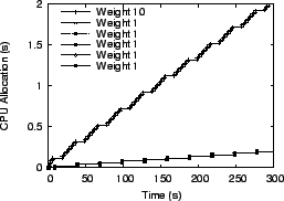
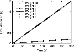
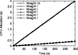
We ran multiple virtual servers with each one having different weights for its processes. In the first experiment, we used six virtual servers, with one server having all its processes assigned weight 10 while all other servers had processes assigned weight 1. In the second experiment, we used five virtual servers and processes assigned to each server had respective weights of 1, 2, 3, 4, and 5. In the third experiment, we ran five virtual servers which assigned a random weight between 1 and 10 to each process. For the Linux scheduler, weights were assigned by selecting nice values appropriately. Figures 14 to 19 present the results from the first experiment with one server with weight 10 processes and all other servers with weight 1 processes. The total load on the system for this experiment consisted of 600 processes running simultaneously. For illustration purposes, only one process from each server is shown in the figures. The conclusions drawn from the other experiments are the same, so other results are not shown due to space constraints.
|
|
| |||
|
|
|
![]() and
and ![]() provided the best overall proportional fairness for
these experiments while Linux provided the worst overall proportional
fairness. Figures 14
to 17 show the amount of processor time allocated to each
client over time for
the Linux scheduler, WFQ, VTRR, and
provided the best overall proportional fairness for
these experiments while Linux provided the worst overall proportional
fairness. Figures 14
to 17 show the amount of processor time allocated to each
client over time for
the Linux scheduler, WFQ, VTRR, and ![]() . All of the schedulers
except
. All of the schedulers
except ![]() and
and ![]() have a pronounced ``staircase'' effect for
the search engine process with weight 10, indicating that CPU resources
are provided in irregular bursts over a short time
interval. For the applications which need to provide interactive
responsiveness to web users, this can result in extra delays in system
response time. It can be inferred from the smoother curves of
Figure 17 that
have a pronounced ``staircase'' effect for
the search engine process with weight 10, indicating that CPU resources
are provided in irregular bursts over a short time
interval. For the applications which need to provide interactive
responsiveness to web users, this can result in extra delays in system
response time. It can be inferred from the smoother curves of
Figure 17 that ![]() and
and ![]() provide fair resource
allocation at a finer granularity than the other schedulers.
provide fair resource
allocation at a finer granularity than the other schedulers.
Fair-share schedulers [12,14,15] provide proportional
sharing among users in a way compatible with a UNIX-style time-sharing
framework based on multi-level feedback with a set of priority queues.
These schedulers typically had low ![]() complexity, but were often
ad-hoc and could not provide any proportional fairness guarantees.
Empirical measurements show that these approaches only provide
reasonable proportional fairness over relatively large time
intervals [12].
complexity, but were often
ad-hoc and could not provide any proportional fairness guarantees.
Empirical measurements show that these approaches only provide
reasonable proportional fairness over relatively large time
intervals [12].
Lottery scheduling [26] gives each client a
number of tickets proportional to its weight, then randomly selects a
ticket.
Lottery scheduling takes ![]() time and
relies on the law of large numbers for providing
proportional fairness. Thus, its allocation errors can be very large,
typically much worse than WRR for clients with smaller weights.
time and
relies on the law of large numbers for providing
proportional fairness. Thus, its allocation errors can be very large,
typically much worse than WRR for clients with smaller weights.
Weighted Fair Queueing (WFQ) [11,18], was first
developed for network packet scheduling, and later applied to
uniprocessor scheduling [26]. It assigns each
client a virtual time and schedules the client with the earliest
virtual time. Other fair queueing variants such as
Virtual-clock [28], SFQ [13],
SPFQ [24], and Time-shift FQ [10]
have also been proposed.
These approaches all have ![]() time complexity, where
time complexity, where ![]() is
the number of clients, because the clients must be ordered by virtual
time. It has been shown that WFQ guarantees that the service time
error for any client never falls below
is
the number of clients, because the clients must be ordered by virtual
time. It has been shown that WFQ guarantees that the service time
error for any client never falls below ![]() [18].
However, WFQ can allow a
client to get far ahead of its ideal allocation and accumulate a large
positive service time error of
[18].
However, WFQ can allow a
client to get far ahead of its ideal allocation and accumulate a large
positive service time error of ![]() , especially with
skewed weight distributions.
, especially with
skewed weight distributions.
Several fair queueing approaches have been proposed for reducing this
![]() service time error. A hierarchical scheduling
approach [26] reduces service time error to
service time error. A hierarchical scheduling
approach [26] reduces service time error to ![]() .
Worst-Case Weighted Fair
Queueing (WF
.
Worst-Case Weighted Fair
Queueing (WF![]() Q) [1] introduced eligible virtual
times and can guarantee both a lower and upper bound on error of
Q) [1] introduced eligible virtual
times and can guarantee both a lower and upper bound on error of ![]() and
and ![]() , respectively for network packet scheduling. It has also
been applied to uniprocessor scheduling as Eligible Virtual Deadline
First (EEVDF) [25].
These algorithms provide stronger proportional fairness guarantees
than other approaches, but are more difficult to implement and still
require at least
, respectively for network packet scheduling. It has also
been applied to uniprocessor scheduling as Eligible Virtual Deadline
First (EEVDF) [25].
These algorithms provide stronger proportional fairness guarantees
than other approaches, but are more difficult to implement and still
require at least ![]() time.
time.
Motivated by the need for faster scheduling algorithms with good
fairness guarantees, one of the authors developed Virtual-Time
Round-Robin (VTRR) [17]. VTRR first introduced the simple
idea of going round-robin through clients but skipping some of them at
different frequencies without having to reorder clients on each
schedule. This is done by combining round-robin scheduling with a
virtual time mechanism. ![]() 's intergroup scheduler builds on VTRR
but uses weight ratios instead of virtual times to provide better
fairness. Smoothed Round Robin (SRR) [9] uses a
different mechanism for skipping clients using a Weight Matrix and
Weight Spread Sequence (WSS) to run clients by simulating a binary
counter. VTRR and SRR provide proportional sharing with
's intergroup scheduler builds on VTRR
but uses weight ratios instead of virtual times to provide better
fairness. Smoothed Round Robin (SRR) [9] uses a
different mechanism for skipping clients using a Weight Matrix and
Weight Spread Sequence (WSS) to run clients by simulating a binary
counter. VTRR and SRR provide proportional sharing with ![]() time
complexity for selecting a client to run, though inserting and
removing clients from the run queue incur higher overhead:
time
complexity for selecting a client to run, though inserting and
removing clients from the run queue incur higher overhead: ![]() for VTRR and
for VTRR and ![]() for SRR , where
for SRR , where
![]() and
and
![]() is the maximum client weight allowed. However, unlike
is the maximum client weight allowed. However, unlike
![]() , both algorithms can suffer from large service time errors
especially for skewed weight distributions. For example, we can show
that the service error of SRR is worst-case
, both algorithms can suffer from large service time errors
especially for skewed weight distributions. For example, we can show
that the service error of SRR is worst-case ![]() .
.
Grouping clients to reduce scheduling complexity has been used
by [20], [8] and
[23]. These fair queueing approaches group
clients into buckets based on client virtual timestamps. With the
exception of [23], which uses exponential
grouping, the fairness of these virtual time bin sorting schemes
depends on the granularity of the buckets and is adversely affected
by skewed client weight distributions. On the other hand, ![]() groups based on client weights, which are relatively static, and uses
groups as schedulable entities in a two-level scheduling
hierarchy.
groups based on client weights, which are relatively static, and uses
groups as schedulable entities in a two-level scheduling
hierarchy.
The grouping strategy used in ![]() was first introduced by two of the
authors for uniprocessor scheduling [6] and generalized by three
of the authors to network packet scheduling [4]. A similar
grouping strategy was independently developed in Stratified Round
Robin (StRR) [19] for network packet scheduling.
StRR distributes all clients with weights between
was first introduced by two of the
authors for uniprocessor scheduling [6] and generalized by three
of the authors to network packet scheduling [4]. A similar
grouping strategy was independently developed in Stratified Round
Robin (StRR) [19] for network packet scheduling.
StRR distributes all clients with weights between ![]() and
and
![]() into class
into class ![]() (
(![]() here not to be confused with our
frontlog). StRR splits time
into scheduling slots and then makes sure to assign all the clients in
class
here not to be confused with our
frontlog). StRR splits time
into scheduling slots and then makes sure to assign all the clients in
class ![]() one slot every scheduling interval, using a credit and
deficit scheme within a class.
This
is also similar to
one slot every scheduling interval, using a credit and
deficit scheme within a class.
This
is also similar to ![]() , with the key difference that a client can
run for up to two consecutive time units, while in
, with the key difference that a client can
run for up to two consecutive time units, while in ![]() , a client is
allowed to run only once every time its group is selected regardless
of its deficit.
, a client is
allowed to run only once every time its group is selected regardless
of its deficit.
StRR has weaker fairness guarantees and higher scheduling
complexity than ![]() . StRR assigns each client weight as a
fraction of the total processing capacity of the system. This results
in weaker fairness guarantees when the sum of these fractions is not
close to the limit of
. StRR assigns each client weight as a
fraction of the total processing capacity of the system. This results
in weaker fairness guarantees when the sum of these fractions is not
close to the limit of ![]() .
For example, if we have
.
For example, if we have ![]() clients, one of weight
clients, one of weight ![]() and the rest of weight
and the rest of weight ![]() (total weight =
(total weight = ![]() ), StRR will run the clients in such a way that after
), StRR will run the clients in such a way that after ![]() slots, the error of the large client is
slots, the error of the large client is ![]() , such that this client will then run uniterruptedly for
, such that this client will then run uniterruptedly for ![]() tu to regain its due service.
Client weights could be
scaled to reduce this error, but with additional
tu to regain its due service.
Client weights could be
scaled to reduce this error, but with additional ![]() complexity.
StRR requires
complexity.
StRR requires ![]() worst-case time to determine the next
class that should be selected, where
worst-case time to determine the next
class that should be selected, where ![]() is the number of groups.
Hardware support can hide this complexity assuming a
small, predefined maximum number of groups [19],
but running an StRR processor scheduler in software still requires
is the number of groups.
Hardware support can hide this complexity assuming a
small, predefined maximum number of groups [19],
but running an StRR processor scheduler in software still requires ![]() complexity.
complexity.
![]() also differs from StRR and other deficit round-robin
variants in its distribution of deficit. In DRR,
SRR, and StRR, the variation in the deficit of all the clients
affects the fairness in the system. To illustrate this, consider
also differs from StRR and other deficit round-robin
variants in its distribution of deficit. In DRR,
SRR, and StRR, the variation in the deficit of all the clients
affects the fairness in the system. To illustrate this, consider ![]() clients, all having the same weight except the first one, whose weight
is
clients, all having the same weight except the first one, whose weight
is ![]() times larger. If the deficit of all the clients except the
first one is close to
times larger. If the deficit of all the clients except the
first one is close to ![]() , the error of the first client will be about
, the error of the first client will be about
![]() . Therefore, the deficit mechanism as
employed in round-robin schemes doesn't allow for better than
. Therefore, the deficit mechanism as
employed in round-robin schemes doesn't allow for better than ![]() error. In contrast,
error. In contrast, ![]() ensures that a group consumes all the
work assigned to it, so that the deficit is a tool used only in
distributing work within a certain group, and not within the
system. Thus, groups effectively isolate the impact of unfortunate
distributions of deficit in the scheduler. This allows for the error
bounds in
ensures that a group consumes all the
work assigned to it, so that the deficit is a tool used only in
distributing work within a certain group, and not within the
system. Thus, groups effectively isolate the impact of unfortunate
distributions of deficit in the scheduler. This allows for the error
bounds in ![]() to depend only on the number of groups instead of the
much larger number of clients.
to depend only on the number of groups instead of the
much larger number of clients.
A rigorous analysis on network packet scheduling
[27] suggests that ![]() delay bounds are
unavoidable with packet scheduling algorithms of less than
delay bounds are
unavoidable with packet scheduling algorithms of less than ![]() time
complexity.
time
complexity.
![]() 's
's ![]() error bound
and
error bound
and ![]() time complexity are consistent with this analysis, since
delay and service error are not equivalent concepts. Thus, if adapted
to packet scheduling,
time complexity are consistent with this analysis, since
delay and service error are not equivalent concepts. Thus, if adapted
to packet scheduling, ![]() would worst-case incur
would worst-case incur ![]() delay while
preserving an
delay while
preserving an ![]() service error.
service error.
Previous work in proportional share scheduling has focused on
scheduling a single resource and little work has been done in
proportional share multiprocessor scheduling. WRR and fair-share
multiprocessor schedulers have been developed, but have the fairness
problems inherent in those approaches. The only multiprocessor fair
queueing algorithm that has been proposed is Surplus Fair Scheduling
(SFS) [7]. SFS also adapts a uniprocessor algorithm,
SFQ, to multiple processors using a centralized
run queue. No theoretical fairness bounds are provided. If a selected
client is already running on another processor, it is removed from
the run queue. This operation may introduce unfairness if used in low
overhead, round-robin variant algorithms. In contrast, ![]() provides strong fairness bounds with lower scheduling overhead.
provides strong fairness bounds with lower scheduling overhead.
SFS introduced the notion of feasible clients along with a
![]() -time weight readjustment algorithm, which requires however
that the clients be sorted by their original weight. By using its
grouping strategy,
-time weight readjustment algorithm, which requires however
that the clients be sorted by their original weight. By using its
grouping strategy, ![]() performs the same weight readjustment in
performs the same weight readjustment in
![]() time without the need to order clients, thus avoiding SFS's
time without the need to order clients, thus avoiding SFS's
![]() overhead per maintenance operation. The optimality of SFS's
and our weight readjustment algorithms rests in preservation of
ordering of clients by weight and of weight proportions among feasible
clients, and not in minimal overall weight change, as [7]
claims.
overhead per maintenance operation. The optimality of SFS's
and our weight readjustment algorithms rests in preservation of
ordering of clients by weight and of weight proportions among feasible
clients, and not in minimal overall weight change, as [7]
claims.
Our experiences with ![]() show
that it is simple to implement and easy to integrate into existing
commodity operating systems. We have measured the performance of
show
that it is simple to implement and easy to integrate into existing
commodity operating systems. We have measured the performance of
![]() using both simulations and kernel measurements of
real system performance using a prototype Linux implementation. Our
simulation results show that
using both simulations and kernel measurements of
real system performance using a prototype Linux implementation. Our
simulation results show that ![]() can provide more than two orders
of magnitude better proportional fairness behavior than other popular
proportional share scheduling algorithms, including WRR, WFQ, SFQ,
VTRR, and SRR. Our experimental results using our
can provide more than two orders
of magnitude better proportional fairness behavior than other popular
proportional share scheduling algorithms, including WRR, WFQ, SFQ,
VTRR, and SRR. Our experimental results using our ![]() Linux
implementation further demonstrate that
Linux
implementation further demonstrate that ![]() provides accurate
proportional fairness behavior on real applications with much lower
scheduling overhead than other Linux schedulers, especially for larger
workloads.
provides accurate
proportional fairness behavior on real applications with much lower
scheduling overhead than other Linux schedulers, especially for larger
workloads.
While small-scale multiprocessors are the most widely available multiprocessor configurations today, the use of large-scale multiprocessor systems is growing given the benefits of server consolidation. Developing accurate, low-overhead proportional share schedulers that scale effectively to manage these large-scale multiprocessor systems remains an important area of future work.
This document was generated using the LaTeX2HTML translator Version 2002-2-1 (1.70)
Copyright © 1993, 1994, 1995, 1996,
Nikos Drakos,
Computer Based Learning Unit, University of Leeds.
Copyright © 1997, 1998, 1999,
Ross Moore,
Mathematics Department, Macquarie University, Sydney.
The command line arguments were:
latex2html -split 0 -show_section_numbers gr3_usenix.tex
The translation was initiated by Bogdan Caprita on 2005-02-16. Document was further editied manually to improve presentation.
Bogdan Caprita
2005-02-16
|
This paper was originally published in the
Proceedings of the 2005 USENIX Annual Technical Conference,
April 10–15, 2005, Anaheim, CA, USA Last changed: 2 Mar. 2005 aw |
|