|
Security '04 Paper
[Security '04 Technical Program]


Static Disassembly of Obfuscated Binaries
Christopher Kruegel, William Robertson, Fredrik Valeur and Giovanni Vigna
Reliable Software Group
University of California Santa Barbara
Abstract:
Disassembly is the process of recovering a symbolic representation of
a program's machine code instructions from its binary
representation. Recently, a number of techniques have been proposed
that attempt to foil the disassembly process. These techniques are
very effective against state-of-the-art disassemblers, preventing a
substantial fraction of a binary program from being disassembled
correctly. This could allow an attacker to hide malicious code from
static analysis tools that depend on correct disassembler output (such
as virus scanners).
The paper presents novel binary analysis techniques that substantially
improve the success of the disassembly process when confronted with
obfuscated binaries. Based on control flow graph information and
statistical methods, a large fraction of the program's instructions
can be correctly identified. An evaluation of the accuracy and the
performance of our tool is provided, along with a comparison to
several state-of-the-art disassemblers.
Keywords: Binary Obfuscation, Reverse Engineering, Static Analysis.
1 Introduction
Software applications are often distributed in binary form to prevent
access to proprietary algorithms or to make tampering with licensing
verification procedures more difficult. The general assumption is that
understanding the structure of a program by looking at its binary
representation is a hard problem that requires substantial resources
and expertise.
Software reverse-engineering techniques provide automated support for
the analysis of binary programs. The goal of these techniques is to
produce a higher-level representation of a program that allows for
comprehension and possibly modification of the program's structure.
The software reverse-engineering process can be divided into two
parts: disassembly and decompilation. The task of the
disassembly phase is the extraction of the symbolic representation of
the instructions (assembly code) from the program's binary
image [12]. Decompilation [5,6]
is the process of reconstructing higher-level semantic structures (and
even source code) from the program's assembly-level representation.
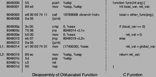
Figure 1:
Example function.
|
A number of approaches have been proposed to make the
reverse-engineering process
harder [8,9,18]. These
techniques are based on transformations that preserve the program's
semantics and functionality and, at the same time, make it more
difficult for a reverse-engineer to extract and comprehend the
program's higher-level structures. The process of applying one or more
of these techniques to an existing program is called obfuscation.
Most previous work on program obfuscation has focused on the
decompilation phase. To this end, researchers have proposed to use
constructs such as indirect jumps or indirect memory references via
pointers that are difficult to
analyze [14,17]. In
[13], Linn and Debray introduce novel obfuscation
techniques that focus on the disassembly phase instead. Their
techniques are independent of and complementary to previous approaches
to make decompilation harder. The main idea is to transform the binary
such that the parsing of instructions becomes difficult. The approach
exploits the fact that the Intel x86 instruction set architecture
contains variable length instructions that can start at arbitrary
memory address. By inserting padding bytes at locations that cannot be
reached during run-time, disassemblers can be confused to misinterpret
large parts of the binary. Although their approach is limited to Intel
x86 binaries, the obfuscation results against current state-of-the-art
disassemblers are remarkable.
Linn and Debray state that their obfuscation techniques can enhance
software security by making it harder for an attacker to steal
intellectual property, to make unauthorized modifications to
proprietary software or to discover vulnerabilities. On the other
hand, program obfuscation could also be used by attackers to hide
malicious code such as viruses or Trojan Horses from virus
scanners [3,16]. Obfuscation also
presents a serious threat to tools that statically analyze binaries to
isolate or to identify malicious
behavior [2,11]. The reason is that if
relevant program structures were incorrectly extracted, malicious code
could be classified as benign.
This paper presents static analysis techniques to correctly
disassemble Intel x86 binaries that are obfuscated to resist static
disassembly. The main contribution are general control-flow-based and
statistical techniques to deal with hard-to-disassemble binaries.
Also, a mechanism is presented that is specifically tailored against
the tool implemented by Linn and Debray [13]. An
implementation based on our approach has been developed, and the
results show that our tool is able to substantially improve the
disassembly of obfuscated binaries.
The paper is structured as follows. In Section 2, the
principal techniques used in binary disassembly are reviewed, together
with a discussion of Linn and Debray's recently proposed obfuscation
techniques. In Section 3, we outline the disassembly
approach and present our assumptions. Section 4 and
Section 5 provide an in-depth description of our disassembly
techniques. In Section 6, a quantitative evaluation of
the accuracy and performance of our disassembler is
presented. Finally, in Section 7, we briefly conclude
and outline future work.
2 Related Work and Background
Disassembly techniques can be categorized into two main classes:
dynamic techniques and static techniques. Approaches that belong to
the first category rely on monitored execution traces of an
application to identify the executed instructions and recover a
(partial) disassembled version of the binary. Approaches that belong
to the second category analyze the binary structure statically,
parsing the instruction opcodes as they are found in the binary image.
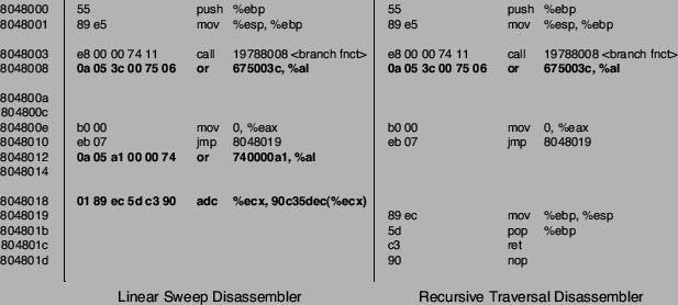
Figure 2:
Traditional disassemblers.
|
Both static and dynamic approaches have advantages and
disadvantages. Static analysis takes into account the complete
program, while dynamic analysis can only operate on the instructions
that were executed in a particular set of runs. Therefore, it is
impossible to guarantee that the whole executable was covered when
using dynamic analysis. On the other hand, dynamic analysis assures
that only actual program instructions are part of the disassembly
output. In this paper, we focus on static analysis techniques only.
In general, static analysis techniques follow one of two
approaches. The first approach, called linear sweep, starts at the
first byte of the binary's text segment and proceeds from there,
decoding one instruction after another. It is used, for example, by
GNU's objdump [10]. The drawback of linear sweep
disassemblers is that they are prone to errors that result from data
embedded in the instruction stream. The second approach, called
recursive traversal, fixes this problem by following the control flow
of the program [6,15]. This
allows recursive disassemblers to circumvent data that is intertwined
with the program instructions. The problem with the second approach is
that the control flow cannot always be reconstructed precisely. When
the target of a control transfer instruction such as a jump or a call
cannot be determined statically (e.g., in case of an indirect jump),
the recursive disassembler fails to analyze parts of the program's
code. This problem is usually solved with a technique called speculative disassembly [4], which uses a linear
sweep algorithm to analyze unreachable code regions.
Linn and Debray's approach [13] to confuse
disassemblers are based on two main techniques. First, junk bytes are
inserted at locations that are not reachable at run-time. These
locations can be found after control transfer instructions such as
jumps where control flow does not continue. Consider the example
in Figure 1, where a function is presented in source form and
in its corresponding assembly representation. At address 0x8048012, two junk bytes are added after the jump instruction at
address 0x8048010. Inserting junk bytes at unreachable locations
should not effect recursive disassemblers, but has a profound impact on
linear sweep implementations.
The second technique relies on a branch function to change the
way regular procedure calls work. This creates more opportunities to
insert junk bytes and misleads both types of disassemblers. A normal
call to a subroutine is replaced with a call to the branch
function. This branch function uses an indirect jump to transfer
control to the original subroutine. In addition, an offset value is
added to the return address of the subroutine. When the subroutine is
done, control is not transfered to the address directly after the call
instruction. Instead, the instruction that is offset number of bytes
after the call instruction is executed. In the example in
Figure 1, two junk bytes are inserted after the call to the
branch function at address 0x8048003. During run-time, the
branch function modifies the return address such that the next
instruction that is executed after the call is at address 0x804800a.
Figure 2 shows the disassembly results for the example
function when using a linear sweep and a recursive traversal
disassembler. The linear sweep disassembler is successfully confused
in both cases where junk bytes are inserted. The two junk bytes at
0x8048008 are interpreted as or instruction, causing the
the following four bytes (which are actually a cmp
and a jne instruction) as being parsed as a
32-bit argument value. A similar problem occurs at address 0x8048012,
resulting in only 5 out of 12 correctly identified instructions.
This recursive disassembler is not vulnerable to the junk bytes
inserted at address 0x8048012 because it recognizes instruction
0x8048010 as an unconditional jump. Therefore, the analysis
can continue at the jump target, which is at address 0x8048019. However, the junk bytes after the call instruction at 0x8048003 lead to incorrect disassembly and the subsequent failure to
decode the jump at 0x804800c with its corresponding target at
0x8048014. In this example, the recursive traversal disassembler
succeeds to correctly identify 9 out of 12 instructions. However, the
situation becomes worse when dealing with real binaries. Because calls
are redirected to the branch function, large parts of the binary
become unreachable for the recursive traversal algorithm. The results
in Section 6 demonstrate that recursive traversal
disassemblers, such as IDA Pro, perform worse on
obfuscated binaries than linear sweep disassemblers, such as objdump.
3 Disassembling Obfuscated Binaries
Our disassembler performs static analysis on Intel x86 binaries. When
analyzing an obfuscated binary, one cannot assume that the code was
generated by a well-behaved compiler. In fact, the obfuscation
techniques introduced by Linn and Debray [13]
precisely exploit the fact that standard disassemblers assume certain
properties of compiler-generated code that can be violated without
changing the program's functionality. By transforming the binary into
functionally equivalent code that does not possess all the assumed
properties, standard disassemblers are confused and fail to correctly
translate binary code into its corresponding assembly representation.
In general, certain properties are easier to change than others and it
is not straightforward to transform (i.e., obfuscate) a binary into a
functionally equivalent representation in which all the
compiler-related properties of the original code are lost. When
disassembling obfuscated binaries, we require that certain assumptions
are valid. These assumptions (some of which constitute limiting
factors for our ability to disassemble obfuscated binaries) are
described in the following subsections.
- Valid instructions must not overlap. An instruction is
denoted as valid if it belongs to the program, that is, it is
reached (and executed) at run-time as part of some legal program
execution trace. Two instructions overlap if one or more bytes
in the executable are shared by both instruction. In other words,
the start of one instruction is located at an address that is
already used by another instruction. Overlapping instructions have
been suggested to complicate disassembly in [7].
However, suitable candidate instructions for this type of
transformation are difficult to find in real executables and the
reported obfuscation effects were minimal [13].
- Conditional jumps can be either taken or not taken. This
means that control flow can continue at the branch target or at the
instruction after the conditional branch. In particular, it is not
possible to insert junk bytes at the branch target or at the address
following the branch instruction. Linn and
Debray [13] discuss the possibility to
transform unconditional jumps into conditional branches using opaque
predicates. Opaque predicates are predicates that always evaluate to
either true or false, independent of the input. This would allow the
obfuscator to insert junk bytes either at the jump target or in
place of the fall-through instruction. However, it is not obvious
how to generate opaque predicates that are not easily recognizable
for the disassembler. Also, the obfuscator presented
in [13] does not implement this transformation.
- An arbitrary amount of junk bytes can be inserted at
unreachable locations. Unreachable locations denotes locations
that are not reachable at run-time. These locations can be found
after instructions that change the normal control flow. For example,
most compilers arrange code such that the address following an
unconditional jump contains a valid instruction. However, we assume
that an arbitrary number of junk bytes can be inserted there.
- The control flow does not have to continue immediately
after a call instruction. Thus, an arbitrary number of padding
bytes can be added after each call. This is different from the
standard behavior where it is expected that the callee returns to
the instruction following a call using the corresponding return
instruction. More specifically, in the x86 instruction set
architecture, the call operation performs a jump to the call
target and, in addition, pushes the address following the call
instruction on the stack. This address is then used by the
corresponding ret instruction, which performs a jump to the
address currently on top of the stack. However, by redirecting calls
to a branch function, it is trivial to change the return address.
Our disassembly techniques can be divided into two classes: general
techniques and tool-specific techniques.
General techniques are techniques that do not rely upon any knowledge
on how a particular obfuscator transforms the binary. It is only
required that the transformations respect our assumptions. Our general
techniques are based on the program's control flow, similar to a
recursive traversal disassembler. However, we use a different approach
to construct the control flow graph, which is more resilient to
obfuscation attempts. Program regions that are not covered by the
control flow graph are analyzed using statistical techniques. The
general techniques are described in more detail in Section 4.
An instance of an obfuscator that respects our assumptions is
presented by Linn and Debray in [13]. By
tailoring the static analysis process against a particular tool, it is
often possible to reverse some of the performed transformations and
improve the analysis results. Section 5 discusses potential
modifications to our general techniques to take advantage of
tool-specific knowledge when disassembling binaries transformed with
Linn and Debray's obfuscator.
In Section 6, we show that the general techniques
presented in the next section offer a significant improvement over
previous approaches. When combined with tool-specific knowledge, the
obfuscated binary is almost completely disassembled.
4 General Techniques
This section discusses the general techniques to reconstruct the
program's control flow. Regions in the binary that are not covered by
the control flow graph are analyzed using statistical methods.
The first step when disassembling obfuscated programs is to divide the
binary into functions that can then be analyzed independently. The
main reason for doing so is run-time performance; it is necessary that
the disassembler scales well enough such that the analysis of large
real-world binaries is possible.
An important part of our analysis is the reconstruction of the
program's control flow. When operating on the complete binary, the
analysis does not scale well for large programs. Therefore, the binary
is broken into smaller regions (i.e., functions) that can be analyzed
consecutively. This results in a run-time overhead of the disassembly
process that is linear in the number of instructions (roughly, the
size of the code segment).
A straightforward approach to obtain a function's start addresses is
to extract the targets of call instructions. When a linker generates
an ordinary executable, the targets of calls to functions located in
the binary's text segment are bound to the actual addresses of these
functions. Given the call targets and assuming that most functions are
actually referenced from others within the binary, one can obtain a
fairly complete set of function start addresses. Unfortunately, this
approach has two drawbacks. One problem is that this method requires
that the call instructions are already identified. As the objective of
our disassembler is precisely to provide that kind of information, the
call instructions are not available at this point. Another problem is
that an obfuscator can redirect all calls to a single branching
function that transfers control to the appropriate targets. This
technique changes all call targets to a single address, thus removing
information necessary to identify functions.
We use a heuristic to locate function start addresses. This is done by
searching the binary for byte sequences that implement typical
function prologs. When a function is called, the first few
instructions usually set up a new stack frame. This frame is required
to make room for local variables and to be able restore the stack to
its initial state when the function returns. In the current
implementation, we scan the binary for byte sequences that represent
instructions that push the frame pointer onto the stack and
instructions that increase the size of the stack by decreasing the
value of the stack pointer. The technique works very well for regular
binaries and also for the obfuscated binaries used in our experiments.
The reason is that the used obfuscation tool [13]
does not attempt to hide function prologs. It is certainly possible to
extend the obfuscator to conceal the function prolog. In this case,
our function identification technique might require changes, possible
using tool-specific knowledge.
Note that the partitioning of the binary into functions is mainly done
for performance reasons, and it is not crucial for the quality of the
results that all functions are correctly identified. When the start
point of a function is missed, later analysis simply has to deal with
one larger region of code instead of two separate smaller parts. When a
sequence of instructions within a function is misinterpreted as a
function prolog, two parts of a single function are analyzed
individually. This could lead to less accurate results when some
intra-procedural jumps are interpreted as inter-procedural, making it
harder to reconstruct the intra-procedural control flow graph as
discussed in the following section.
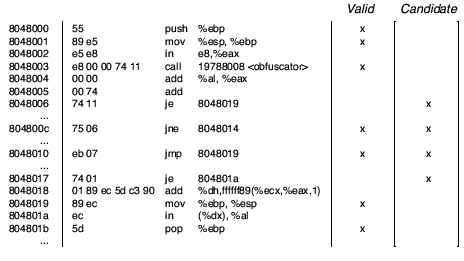
Figure 3:
Partial instruction listing.
|
4.2 Intra-Procedural Control Flow Graph
To find the valid instructions of a function (i.e., the instructions
that belong to the program), we attempt to reconstruct the function's
intra-procedural control flow graph. A control flow graph (CFG) is
defined as a directed graph  in which vertices in which vertices  represent basic blocks and an edge
 represents a possible flow of control from
  to to  . A basic block
describes a sequence of instructions without any jumps or jump targets
in the middle. More formally, a basic block is defined as a sequence
of instructions where the instruction in each position dominates, or
always executes before, all those in later positions, and no other
instruction executes between two instructions in the
sequence. Directed edges between blocks represent jumps in the control
flow, which are caused by control transfer instructions (CTIs) such as
calls, conditional and unconditional jumps, or return instructions. . A basic block
describes a sequence of instructions without any jumps or jump targets
in the middle. More formally, a basic block is defined as a sequence
of instructions where the instruction in each position dominates, or
always executes before, all those in later positions, and no other
instruction executes between two instructions in the
sequence. Directed edges between blocks represent jumps in the control
flow, which are caused by control transfer instructions (CTIs) such as
calls, conditional and unconditional jumps, or return instructions.
The traditional approach to reconstruct the control flow graph of a
function works similar to a recursive disassembler. The analysis
commences at the function's start address and instructions are
disassembled until a control transfer instruction is encountered. The
process is then continued recursively at all jump targets that are
local to the procedure and, in case of a call instruction or a
conditional jump, at the address following the instruction. In case of
an obfuscated binary, however, the disassembler cannot continue
directly after a call instruction. In addition, many local jumps are
converted into non-local jumps to addresses outside the function to
blur local control flow. In most cases, the traditional approach leads
to a control flow graph that covers only a small fraction of the valid
instructions of the function under analysis. This claim is supported
by the experimental data shown in Section 6 that
includes the results for a state-of-the-art recursive disassembler.
We developed an alternative technique to extract a more complete
control flow graph. The technique is composed of two phases: in the
first phase, an initial control flow graph is determined. In the
following phase, conflicts and ambiguities in the initial CFG are
resolved. The two phases are presented in detail in the next two
sections.
To determine the initial control flow graph for a function, we first
decode all possible instructions between the function's start and end
addresses. This is done by treating each address in this address range
as the begin of a new instruction. Thus, one potential instruction is
decoded and assigned to each address of the function. The reason for
considering every address as a possible instruction start stems from
the fact that x86 instructions have a variable length from one to
fifteen bytes and do not have to be aligned in memory (i.e., an
instruction can start at an arbitrary address). Note that most
instructions take up multiple bytes and such instructions overlap with
other instructions that start at subsequent bytes. Therefore, only a
subset of the instructions decoded in this first step can be
valid. Figure 3 provides a partial listing of all
instructions in the address range of the sample function that is shown
in Figure 1. For the reader's reference, valid instructions
are marked by an x in the ``Valid'' column. Of course,
this information is not available to our disassembler. An example for
the overlap between valid and invalid instructions can be seen between
the second and the third instruction. The valid instruction at address
0x8048001 requires two bytes and thus interferes with the next
(invalid) instruction at 0x8048002.
The next step is to identify all intra-procedural control transfer
instructions. For our purposes, an intra-procedural control transfer
instruction is defined as a CTI with at least one known successor
basic block in the same function. Remember that we assume that control
flow only continues after conditional branches but not necessarily
after call or unconditional branch instructions. Therefore, an
instruction is an intra-procedural control transfer instruction if
either (i) its target address can be determined and this address
is in the range between the function's start and end addresses or (ii) it is a conditional jump.
Note that we assume that a function is represented by a contiguous
sequence of instructions, with possible junk instructions added in
between. However, it is not possible that the basic blocks of two
different functions are intertwined. Therefore, each function has one
start address and one end address (i.e., the last instruction of the
last basic block that belongs to this function). However, it is
possible that a function has multiple exit points.
In case of a conditional jump, the address that immediately follows
the jump instruction is the start of a successor block, and thus,
every conditional jump is also an intra-procedural control transfer
operation. This is intuitively plausible, as conditional branches are
often used to implement local branch (e.g., if-else) and loop
(e.g., while, for) statements of higher-level languages,
such as C.
To find all intra-procedural CTIs, the instructions decoded in the
previous step are scanned for any control transfer instructions. For
each CTI found in this way, we attempt to extract its target
address. In the current implementation, only direct address modes are
supported and no data flow analysis is performed to compute address
values used by indirect jumps. However, such analysis could be later
added to further improve the performance of our static analyzer. When
the instruction is determined to be an intra-procedural control
transfer operation, it is included in the set of jump
candidates. The jump candidates of the sample function are marked in
Figure 3 by an x in the ``Candidate'' column. In
this example, the call at address 0x8048003 is not included into
the set of jump candidates because the target address is located
outside the function.
Given the set of jump candidates, an initial control flow graph is
constructed. This is done with the help of a recursive
disassembler. Starting with an initial empty CFG, the disassembler is
successively invoked for all the elements in the set of jump
candidates. In addition, it is also invoked for the instruction at
the start address of the function.
The key idea for taking into account all possible control transfer
instructions is the fact that the valid CTIs determine the skeleton of
the analyzed function. By using all control flow instructions to
create the initial CFG, we make sure that the real CFG is a subgraph
of this initial graph. Because the set of jump candidates can contain
both valid and invalid instructions, it is possible (and also
frequent) that the initial CFG contains a superset of the nodes of the
real CFG. These nodes are introduced as a result of argument bytes of
valid instructions being misinterpreted as control transfer
instructions. The Intel x86 instruction set contains 26 single-byte
opcodes that map to control transfer instructions (out of 219
single-byte instruction opcodes). Therefore, the probability that a
random argument byte is decoded as CTI is not negligible. In our
experiments (for details, see Section 6), we found that
about one tenth of all decoded instructions are CTIs. Of those
instructions, only two thirds were part of the real control flow
graph. As a result, the initial CFG contains nodes and edges that
represent invalid instructions. Most of the time, these nodes contain
instructions that overlap with valid instructions of nodes that belong
to the real CFG. The following section discusses mechanisms to remove
these spurious nodes from the initial control flow graph. It is
possible to distinguish spurious from valid nodes because invalid CTIs
represent random jumps within the function while valid CTIs constitute
a well-structured CFG with nodes that have no overlapping
instructions.
Creating an initial CFG that includes nodes that are not part of the
real control flow graph can been seen as the opposite to the operation
of a recursive disassembler. A standard recursive disassembler starts
from a known valid block and builds up the CFG by adding nodes as it
follows the targets of control transfer instructions that are
encountered. This technique seems favorable at first glance, as it
makes sure that no invalid instructions are incorporated into the
CFG. However, most control flow graphs are partitioned into several
unconnected subgraphs. This happens because there are control flow
instructions such as indirect branches whose targets often cannot be
determined statically. This leads to missing edges in the CFG and to
the problem that only a fraction of the real control flow graph is
reachable from a certain node. The situation is exacerbated when
dealing with obfuscated binaries, as inter-procedural calls and jumps
are redirected to a branching function that uses indirect jumps. This
significantly reduces the parts of the control flow graph that are
directly accessible to a recursive disassembler, leading to
unsatisfactory results.
Although the standard recursive disassembler produces suboptimal
results, we use a similar algorithm to extract the basic blocks to
create the initial CFG. As mentioned before, however, the recursive
disassembler is not only invoked for the start address of the function
alone, but also for all jump candidates that have been identified. An
initial control flow graph is then constructed according to the
code listing shown in Algorithm 1.
![\begin{algorithm}
% latex2html id marker 149
[h]
\Setnlsty{textsf}{L}{:}
\AlgRes...
...n(inst);
}}
}
return current\;
\caption{\textsf{disassemble()}}
\end{algorithm}](img9.png)
There are two differences between a standard recursive disassembler
and our implementation. First, we assume that the address after a call
or an unconditional jump instruction does not have to contain a valid
instruction. Therefore, our recursive disassembler cannot continue at
the address following a call or an unconditional jump. Note, however,
that we do continue to disassemble after a conditional jump (i.e.,
branch). This can be seen at Label 5 of Algorithm 1
where the disassembler recursively continues after conditional branch
instructions.
The second difference is due to the fact that it is possible to have
instructions in the initial call graph that overlap. In this case, two
different basic blocks in the call graph can contain overlapping
instructions starting at slightly different addresses. When following
a sequence of instructions, the disassembler can arrive at an
instruction that is already part of a previously found basic block. In
the regular case, this instruction is the first instruction of the
existing block. The disassembler can complete the instruction sequence
of the current block and create a link to the existing basic block in
the control flow graph.
When instructions can overlap, it is possible that the current
instruction sequence starts to overlap with another sequence in an
existing basic block for some instructions before the two sequences
eventually merge. At the point where the two sequences merge, the
disassembler finds an instruction that is in the middle (or at the
end) of a sequence associated with an existing basic block. In this
case, the existing basic block is split into two new blocks. One block
refers to the overlapping sequence up to the instruction where the two
sequences merge, the other refers to the instruction sequence that
both have in common. All edges in the control flow graph that point to
the original basic block are changed to point to the first block,
while all outgoing edges of the original block are assigned to the
second. In addition, the first block is connected to the second
one. The reason for splitting the existing block is the fact that a
basic block is defined as a continuous sequence of instructions without
a jump or jump target in the middle. When two different overlapping
sequences merge at a certain instruction, this instruction has two
predecessor instructions (one in each of the two overlapping
sequences). Therefore, it becomes the first instruction of a new basic
block. As an additional desirable side effect, each instruction
appears at most once in a basic block of the call graph.
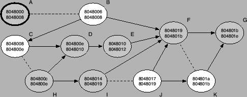
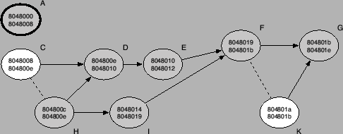
Figure 4:
Initial control flow graph.
|
The functionality of splitting an existing basic block is implemented
by the split procedure referenced at Label 3 of
Algorithm 1. Whenever an instruction is found that is already
associated with a basic block (check performed at Label 1),
the instruction sequence of the current basic block is completed. When
the instruction is in the middle of the existing block (check
performed at Label 2), it is necessary to split the
block. The current block is then connected either to the existing
basic block or, after a split, to the newly created block that
contains the common instruction sequence. The check performed at
Label 4 takes care of the special case where the recursive
disassembler starts with an instruction that is part of an existing
basic block. In this case, the current block contains no instructions
and a reference to the old block is returned instead.
The situation of two merging instruction sequences is a common
phenomenon when disassembling x86 binaries. The reason is called self-repairing disassembly and relates to the fact that two
instruction sequences that start at slightly different addresses (that
is, shifted by a few bytes) synchronize quickly, often after a few
instructions. Therefore, when the disassembler starts at an address
that does not correspond to a valid instruction, it can be expected
to re-synchronize with the sequence of valid instructions after
a few steps [13].
The initial control flow graph that is created by Algorithm 1
for our example function is shown in Figure 4. In this
example, the algorithm is invoked for the function start at address
0x8048000 and the four jump candidates (0x8048006, 0x804800c, 0x8048010, and 0x8048017). The nodes in this
figure represent basic blocks and are labeled with the start address
of the first instruction and the end address of the last instruction
in the corresponding instruction sequence. Note that the end address
denotes the first byte after the last instruction and is not
part of the basic block itself. Solid, directed edges between nodes
represent the targets of control transfer instructions. A dashed line
between two nodes signifies a conflict between the two
corresponding blocks. Two basic blocks are in conflict when they
contain at least one pair of instructions that overlap. As discussed
previously, our algorithm guarantees that a certain instruction is
assigned to at most one basic block (otherwise, blocks are split
appropriately). Therefore, whenever the address ranges of two blocks
overlap, they must also contain different, overlapping
instructions. Otherwise, both blocks would contain the same
instruction, which is not possible. This is apparent in
Figure 4, where the address ranges of all pairs of
conflicting basic blocks overlap. To simplify the following discussion
of the techniques used to resolve conflicts, nodes that belong to the real
control flow graph are shaded. In addition, each node is denoted with
an uppercase letter.
4.2.2 Block Conflict Resolution
The task of the block conflict resolution phase is to remove basic
blocks from the initial CFG until no conflicts are present
anymore. Conflict resolution proceeds in five steps. The first two
steps remove blocks that are definitely invalid, given our
assumptions. The last three steps are heuristics that choose likely invalid blocks. The conflict resolution phase terminates
immediately after the last conflicting block is removed; it is not
necessary to carry out all steps. The final step brings about a
decision for any basic block conflict and the control flow graph is
guaranteed to be free of any conflicts when the conflict resolution
phase completes.
The five steps are detailed in the following paragraphs.
Figure 5:
CFG after two steps of conflict resolution.
|
Step 1: We assume that the start address of the
analyzed function contains a valid instruction. Therefore, the basic
block that contains this instruction is valid. In addition, whenever a
basic block is known to be valid, all blocks that are reachable from
this block are also valid.
A basic block is reachable from basic block if there
exists a path  from to . A path from to is
defined as a sequence of edges that begins at and terminates at
. An edge is inserted into the control flow graph only when its
target can be statically determined and a possible program execution
trace exists that transfers control over this edge. Therefore,
whenever a control transfer instruction is valid, its targets have to
be valid as well. from to . A path from to is
defined as a sequence of edges that begins at and terminates at
. An edge is inserted into the control flow graph only when its
target can be statically determined and a possible program execution
trace exists that transfers control over this edge. Therefore,
whenever a control transfer instruction is valid, its targets have to
be valid as well.
We tag the node that contains the instruction at the function's start
address and all nodes that are reachable from this node as valid. Note
that this set of valid nodes contains exactly the nodes that a
traditional recursive disassembler would identify when invoked with
the function's start address. When the valid nodes are identified, any
node that is in conflict with at least one of the valid nodes can be
removed.
In the initial control flow graph for the example function in
Figure 4, only node A (0x8048000) is marked as
valid. That node is drawn with a stronger border in
Figure 4. The reason is that the corresponding basic block
ends with a call instruction at 0x8048003 whose target is not
local. In addition, we do not assume that control flow resumes at the
address after a call and thus the analysis cannot directly continue
after the call instruction. In Figure 4, node B (the basic
block at 0x8048006) is in conflict with the valid node
and can be removed.
Step 2: Because of the assumption that valid
instructions do not overlap, it is not possible to start from a valid
block and reach two different nodes in the control flow graph that are
in conflict. That is, whenever two conflicting nodes are both
reachable from a third node, this third node cannot be valid and is
removed from the CFG. The situation can be restated using the notion
of a common ancestor node. A common ancestor node of two nodes and
is defined as a node  such that both and are reachable
from . such that both and are reachable
from .
In Step 2, all common ancestor nodes of conflicting nodes are removed
from the control flow graph. In our example in Figure 4, it
can be seen that the conflicting node F and node K share a common
ancestor, namely node J. This node is removed from the CFG, resolving
a conflict with node I. The resulting control flow graph after the
first two steps is shown in Figure 5.
The situation of having a common ancestor node of two conflicting
blocks is frequent when dealing with invalid conditional branches. In
such cases, the branch target and the continuation after the branch
instruction are often directly in conflict, allowing one to remove the
invalid basic block from the control flow graph.
Step 3: When two basic blocks are in conflict, it is
reasonable to expect that a valid block is more tightly integrated
into the control flow graph than a block that was created because of a
misinterpreted argument value of a program instruction. That means
that a valid block is often reachable from a substantial number of
other blocks throughout the function, while an invalid block usually
has only a few ancestors.
The degree of integration of a certain basic block into the control
flow graph is approximated by the number of its predecessor nodes. A
node is defined as a predecessor node of when is
reachable by . In Step 3, the predecessor nodes for pairs of
conflicting nodes are determined and the node with the smaller number
is removed from the CFG.
In Figure 5, node K has no predecessor nodes while node F has
five. Note that the algorithm cannot distinguish between real and
spurious nodes and thus includes node C in the set of predecessor
nodes for node F. As a result, node K is removed. The number of
predecessor nodes for node C and node H are both zero and no decision
is made in the current step.
Step 4: In this step, the number of direct successor
nodes of two conflicting nodes are compared. A node is a direct successor node of node when can be directly reached
through an outgoing edge from . The node with less direct successor
nodes is then removed. The rationale behind preferring the node with
more outgoing edges is the fact that each edge represents a jump
target within the function and it is more likely that a valid control
transfer instruction has a target within the function than any random
CTI.
In Figure 5, node C has only one direct successor node while
node H has two. Therefore, node C is removed from the control flow
graph. In our example, all conflicts are resolved at this point.
Step 5: In this step, all conflicts between basic
blocks must be resolved. For each pair of conflicting blocks, one is
chosen at random and then removed from the graph. No human
intervention is required at this step, but it would be possible to
create different alternative disassembly outputs (one output for each
block that needs to be removed) that can be all presented to a human
analyst.
It might also be possible to use statistical methods during Step 5 to
improve the chances that the ``correct'' block is selected. However,
this technique is not implemented and is left for future work.
The result of the conflict resolution step is a control flow graph
that contains no overlapping basic blocks. The instructions in these
blocks are considered valid and could serve as the output of the
static analysis process. However, most control flow graphs do not
cover the function's complete address range and gaps exist between
some basic blocks.
The task of the gap completion phase is to improve the results of our
analysis by filling the gaps between basic blocks in the control flow
graph with instructions that are likely to be valid. A gap from
basic block  to basic block to basic block  is the sequence of addresses
that starts at the first address after the end of basic block
and ends at the last address before the start of block , given
that there is no other basic block in the control flow graph that
covers any of these addresses. In other words, a gap contains bytes
that are not used by any instruction in the control flow graph. is the sequence of addresses
that starts at the first address after the end of basic block
and ends at the last address before the start of block , given
that there is no other basic block in the control flow graph that
covers any of these addresses. In other words, a gap contains bytes
that are not used by any instruction in the control flow graph.
Gaps are often the result of junk bytes that are inserted by the
obfuscator. Because junk bytes are not reachable at run-time, the
control flow graph does not cover such bytes. It is apparent that the
attempt to disassemble gaps filled with junk bytes does not improve
the results of the analysis. However, there are also gaps that do
contain valid instructions. These gaps can be the result of an
incomplete control flow graph, for example, stemming from a region of
code that is only reachable through an indirect jump whose target
cannot be determined statically. Another frequent cause for gaps that
contain valid instructions are call instructions. Because the
disassembler cannot continue after a call instruction, the following
valid instructions are not immediately reachable. Some of these
instructions might be included into the control flow graph because
they are the target of other control transfer instructions. Those
regions that are not reachable, however, cause gaps that must be
analyzed in the gap completion phase.
The algorithm to identify the most probable instruction sequence in a
gap from basic block to basic block works as
follows. First, all possibly valid sequences in the gap are
identified. A necessary condition for a valid instruction sequence is
that its last instruction either (i) ends with the last byte of
the gap or (ii) its last instruction is a non intra-procedural
control transfer instruction. The first condition states that the last
instruction of a valid sequence has to be directly adjacent to the
first instruction of the second basic block . This becomes
evident when considering a valid instruction sequence in the gap that
is executed at run-time. After the last instruction of the sequence
is executed, the control flow has to continue at the first
instruction of basic block . The second condition states that a
sequence does not need to end directly adjacent to block if the
last instruction is a non intra-procedural control transfer. The
restriction to non intra-procedural CTIs is necessary because all
intra-procedural CTIs are included into the initial control flow
graph. When an intra-procedural instruction appears in a gap, it must
have been removed during the conflict resolution phase and should not
be included again.
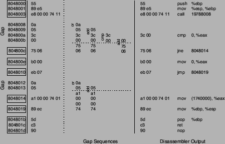
Figure 6:
Gap completion and disassembler output.
|
Instruction sequences are found by considering each byte between the
start and the end of the gap as a potential start of a valid
instruction sequence. Subsequent instructions are then decoded until the
instruction sequence either meets or violates one of the necessary
conditions defined above. When an instruction sequence meets a
necessary condition, it is considered possibly valid and a sequence score is calculated for it. The sequence score is a measure
of the likelihood that this instruction sequence appears in an
executable. It is calculated as the sum of the instruction
scores of all instructions in the sequence. The instruction score is
similar to the sequence score and reflects the likelihood of an
individual instruction. Instruction scores are always greater or equal
than zero. Therefore, the score of a sequence cannot decrease when
more instructions are added. We calculate instruction scores using
statistical techniques and heuristics to identify improbable
instructions.
The statistical techniques are based on instruction probabilities and
digraphs. Our approach utilizes tables that denote both the likelihood
of individual instructions appearing in a binary as well as the
likelihood of two instructions occurring as a consecutive pair. The
tables were built by disassembling a large set of common executables
and tabulating counts for the occurrence of each individual
instruction as well as counts for each occurrence of a pair of
instructions. These counts were subsequently stored for later use
during the disassembly of an obfuscated binary. It is important to
note that only instruction opcodes are taken into account with this
technique; operands are not considered. The basic score for a
particular instruction is calculated as the sum of the probability
of occurrence of this instruction and the probability of occurrence
of this instruction followed by the next instruction in the sequence.
In addition to the statistical technique, a set of heuristics are used
to identify improbable instructions. This analysis focuses on
instruction arguments and observed notions of the validity of certain
combinations of operations, registers, and accessing modes. Each
heuristic is applied to an individual instruction and can modify the
basic score calculated by the statistical technique. In our current
implementation, the score of the corresponding instruction is set to
zero whenever a rule matches. Examples of these rules include the
following:
- operand size mismatches;
- certain arithmetic on special-purpose registers;
- unexpected register-to-register moves
(e.g., moving from a register other than %ebp into %esp);
- moves of a register value into memory referenced by
the same register.
When all possible instruction sequences are determined, the one with the
highest sequence score is selected as the valid instruction sequence
between and .
The instructions that make up the control flow graph of our example
function and the intermediate gaps are shown in the left part of
Figure 6. It can be seen that only a single instruction
sequence is valid in the first gap, while there is none in the second
gap. The right part of Figure 6 shows the output of our
disassembler. All valid instructions of the example function have been
correctly identified.
5 Tool-Specific Techniques
The techniques discussed in the previous section can disassemble any
binary that satisfies our assumptions with reasonable accuracy (see
Section 6 for detailed results). As mentioned
previously, however, the results can be improved when taking advantage
of available tool-specific knowledge. This section introduces a
modification to our general techniques that can be applied when
disassembling binaries transformed with Linn and Debray's obfuscator.
A significant problem for the disassembler is the fact that it cannot
continue disassembling at the address following a call instruction. As
discussed in Section 2, Linn and Debray's obfuscator
replaces regular calls with calls to a branch function. The
branch function is responsible for determining the real call target,
that is, the function that is invoked in the original program. This is
done using a perfect hash function, using the location of
the call instruction as input. During run-time, the location of the
call instruction can be conveniently determined from the top of the
stack. The reason is that the address following the call instruction
is pushed on the stack by the processor as part of the x86
call operation.
Besides finding the real target of the call and jumping to the
appropriate address, the branch function is also responsible for
adjusting the return address such that control flow does not return
directly to the address after the call instruction. This is achieved
by having the branch function add a certain offset to the return
address on the stack. This offset is constant (but possibly different) for
each call instruction and obtained in a way similar to the target
address by performing a table lookup based on the location of the
caller. When the target function eventually returns using the
modified address on the stack, the control flow is transfered to an
instruction located at offset bytes after the original return
address. This allows the obfuscator to fill these bytes with junk.
By reverse engineering the branch function, the offset can be
statically determined for each call instruction. This allows the
disassembler to skip the junk bytes and continue at the correct
instruction. One possibility is to manually reverse engineer the
branch function for each obfuscated binary. However, the process is
cumbersome and error prone. A preferred alternative is to
automatically extract the desired information.
We observe that the branch function is essentially a procedure that
takes one input parameter, which is the address after the call
instruction that is passed on the top of the stack. The procedure then
returns an output value by adjusting this address on the stack. The
difference between the initial value on the stack and the modified
value is the offset that we are interested in. It is easy to simulate
the branch function because its output only depends on the single
input parameter and several static lookup tables that are all present
in the binary's initialized data segment. As the output does not
depend on any input the program receives during run-time, it can be
calculated statically.
To this end, we have implemented a simple virtual processor as part of
the disassembler that simulates the instructions of the branch
function. Because the branch function does not depend on dynamic
input, all memory accesses refer to addresses in the initialized data
segment and can be satisfied statically. The execution environment is
set up such that the stack pointer of the virtual processor points to
an address value for which we want to determine the offset. Then, the
simulator executes instructions until the input address value on the
stack is changed. At this point, the offset for a call is
calculated by subtracting the old address value from the new one.
Whenever the disassembler encounters a call instruction, the value of
the address following the call is used to invoke our branch function
simulator. The simulator calculates the corresponding offset, and the
disassembler can then skip the appropriate number of junk bytes to
continue at the next valid instruction.
6 Evaluation
Linn and Debray evaluated their obfuscation tool using the SPECint 95
benchmark suite, a set of eight benchmark applications written in
C. These programs were compiled with gcc version egcs-2.91.66 at optimization level -O3 and then obfuscated.
Table 1:
Disassembler accuracy.
| |
|
|
|
Our tool |
| |
|
| compress95 |
56.07 |
69.96 |
24.19 |
91.04 |
98.07 |
| gcc |
65.54 |
82.18 |
45.09 |
88.45 |
95.17 |
| go |
66.08 |
78.12 |
43.01 |
91.81 |
96.80 |
| ijpeg |
60.82 |
74.23 |
31.46 |
91.60 |
97.53 |
| li |
56.65 |
72.78 |
29.07 |
89.86 |
97.35 |
| m88ksim |
58.42 |
75.66 |
29.56 |
90.39 |
97.49 |
| perl |
57.66 |
72.01 |
31.36 |
86.93 |
96.28 |
| vortex |
66.02 |
76.97 |
42.65 |
90.71 |
96.65 |
| Mean |
60.91 |
75.24 |
34.55 |
90.10 |
96.92 |
|
To measure the efficacy of the obfuscation process, the confusion factor for instructions was introduced. This metric
measures how many program instructions were incorrectly
disassembled. More formally, let V be the set of valid program
instructions and O the set of instructions that a disassembler
outputs. Then, the confusion factor CF is defined as
 . Because our work focuses on the efficacy of the
disassembler in identifying valid instructions, we define the disassembler accuracy DA as . Because our work focuses on the efficacy of the
disassembler in identifying valid instructions, we define the disassembler accuracy DA as
 . .
Linn and Debray used three different disassemblers to evaluate the
quality of their obfuscator. The first one was the GNU objdump
utility, which implements a standard linear sweep algorithm. The
second disassembler was implemented by Linn and Debray themselves. It
is a recursive disassembler that uses speculative linear disassembly
(comparable to our gap completion) for regions that are not reachable by
the recursive part. This disassembler was also provided with
additional information about the start and end addresses of all
program functions. The purpose of this disassembler was to serve as
an upper bound estimator for the disassembler accuracy and to avoid
reporting ``unduly optimistic results'' [13]. The
third disassembler was IDA Pro 4.3x, a commercial
disassembler that is often considered to be among the best
commercially available disassemblers. This belief is also reflected in
the fact that IDA Pro is used to provide disassembly as
input for static analysis tools such as [3].
We developed a disassembler that implements the general techniques and
the tool-specific modification presented in the two previous
sections. Our tool was then run on the eight obfuscated SPECint 95
applications. The results for our tool and a comparison to the three
disassemblers used by Linn and Debray are shown in
Table 1. Note that we report two results for our
disassembler. One shows the disassembler accuracy when only general
techniques are utilized. The second result shows the disassembler
accuracy when the tool-specific modification is also enabled.
These results demonstrate that our disassembler provides a significant
improvement over the best disassembler used in the evaluation by Linn
and Debray. Even without using tool-specific knowledge, the
disassembler accuracy is higher than their recursive disassembler used
to estimate the upper bound for the disassembler accuracy. When the
tool-specific modification is enabled, the binary is disassembled
almost completely. The poor results for IDA Pro can be
explained with the fact that the program only disassembles addresses
that can be guaranteed (according to the tool) to be instructions. As a
result, many functions that are invoked through the branch function
are not disassembled at all. In addition, IDA Pro
continues directly after call instructions and is frequently mislead
by junk bytes there.
Given the satisfying results of our disassembler, the disassembly
process was analyzed in more detail. It is interesting to find the
ratio between the number of valid instructions identified by the
control flow graph and the number of valid instructions identified by
the gap completion phase. Although the gap completion phase is
important in filling regions not covered by the CFG, our key
observation is the fact that the control transfer instructions and the
resulting control flow graph constitute the skeleton of an analyzed
function. Therefore, one would expect that most valid instructions can
be derived from the control flow graph, and only small gaps (e.g.,
caused by indirect calls or unconditional jumps) need to be completed
later. Table 2 shows the fraction (in percent) of
correctly identified, valid instructions that were obtained using the
control flow graph and the fraction obtained in the gap completion
phase. Because the numbers refer to correctly identified instructions
only, the two fractions sum up to unity. Both the results with
tool-specific support and the results with the general techniques
alone are provided. When tool specific support is available, the
control flow graph contributes noticeable more to the output. In this
case, the disassembler can include all regions following call
instructions into the CFG. However, in both experiments, a clear
majority of the output was derived from the control flow graph,
confirming our key observation.
Table 2:
CFG vs. gap completion.
| |
general |
tool-specific |
| |
CFG |
Gap |
CFG |
| compress95 |
87.09 |
12.91 |
96.36 |
3.64 |
| gcc |
85.12 |
14.88 |
93.10 |
6.90 |
| go |
89.13 |
10.87 |
95.11 |
4.89 |
| ijpeg |
87.02 |
12.98 |
95.03 |
4.97 |
| li |
85.63 |
14.37 |
95.11 |
4.89 |
| m88ksim |
87.18 |
12.82 |
96.00 |
4.00 |
| perl |
86.22 |
13.78 |
95.57 |
4.43 |
| vortex |
88.04 |
11.96 |
94.67 |
5.33 |
| Mean |
86.93 |
13.07 |
95.12 |
4.88 |
|
Table 3:
Conflict resolution.
| |
|
Conflict Resolution |
|
| |
|
Step 1 |
Step 2 |
Step 3 |
| compress95 |
54674 |
7021 |
4693 |
4242 |
93 |
48 |
38577 |
| gcc |
245586 |
21762 |
25680 |
29801 |
900 |
565 |
166878 |
| go |
91140 |
10667 |
8934 |
9405 |
231 |
154 |
61749 |
| ijpeg |
70255 |
9414 |
6069 |
5299 |
140 |
95 |
49238 |
| li |
63459 |
8350 |
5297 |
4952 |
125 |
78 |
44657 |
| m88ksim |
77344 |
10061 |
6933 |
6938 |
177 |
101 |
53134 |
| perl |
104841 |
10940 |
11442 |
11750 |
291 |
152 |
70266 |
| vortex |
118703 |
15004 |
9221 |
13424 |
407 |
373 |
80274 |
|
Because most of the output is derived from the control flow graph, it
is important that the conflict resolution phase is effective. One
third of the control transfer instructions that are used to create the
initial control flow graphs are invalid. To achieve a good
disassembler accuracy, it is important to remove the invalid nodes
from the CFG. The first two steps of the conflict resolution phase
remove nodes that are guaranteed to be invalid, given our
assumptions. The third and forth step implement two heuristics and the
fifth step randomly selects one of two conflicting nodes. It is
evident that it is desirable to have as many conflicts as possible
resolved by the first and second step, while the fifth step should
never be required.
Table 3 shows for each program the number of basic blocks
in the initial control flow graphs (column Initial Blocks) and
the number of basic blocks in the control flow graphs after the
conflict resolution phase (column Final Blocks). In addition,
the number of basic blocks that were removed in each of the five steps
of the conflict resolution phase are shown. The numbers given in
Table 3 were collected when the tool-specific
modification was enabled. The results were very similar when only
general techniques were used.
It can be seen that most conflicts were resolved after the first three
steps. About two thirds of the removed basic blocks were guaranteed to
be invalid. This supports our claim that invalid control flow
instructions, caused by the misinterpretation of instruction
arguments, often result in impossible control flows that can be easily
detected. Most of the remaining blocks are removed by the first
heuristic that checks how tight a block is connected with the rest of
the CFG. Invalid blocks are often loosely coupled and can taken out
during this step. The last two steps were only responsible for a small
fraction of the total removed blocks. The heuristic in step four was
sometimes able to provide an indication of which block was
valid. Otherwise, a random node had to be selected.
Static analysis tools are traditionally associated with poor
scalability and the inability to deal with real-world
input. Therefore, it is important to ascertain that our disassembler
can process even large real-world binaries in an acceptable amount of
time. In Section 4, we claimed that the processing
overhead of the program is linear in the number of instructions of the
binary. The intuitive reason is the fact that the binary is
partitioned into functions that are analyzed independently. Assuming
that the average size of an individual function is relatively
independent of the size of the binary, the amount of work per function
is also independent of the size of the binary. As a result, more
functions have to be analyzed as the size of the binary
increases. Because the number of functions increases linearly with the
number of instructions and the work per function is constant (again,
assuming a constant average function size), the overhead of the static
analysis process is linear in the number of instructions.
Table 4:
Disassembler processing times.
| Program |
Size (Bytes) |
Instructions |
Time (s) |
| openssh |
263,684 |
46,343 |
4 |
| compress95 |
1,768,420 |
92,137 |
9 |
| li |
1,820,768 |
109,652 |
7 |
| ijpeg |
1,871,776 |
127,012 |
9 |
| m88ksim |
2,001,616 |
127,358 |
8 |
| go |
2,073,728 |
145,953 |
11 |
| perl |
2,176,268 |
169,054 |
15 |
| vortex |
2,340,196 |
204,230 |
16 |
| gcc |
2,964,740 |
387,289 |
28 |
| emacs |
4.765,512 |
405,535 |
38 |
|
To support this claim with experimental data, the time for a complete
disassembly of each evaluation binary was taken. The size of
obfuscated programs of the SPECint 95 benchmark are in the range of
1.77 MB to 2.96 MB. To obtain more diversified results, we also
disassembled one smaller (openssh 3.7) and one larger
binary (emacs 21.3). The processing times were taken as
the average of ten runs on a 1.8 GHz Pentium IV system
with 512 MB of RAM, running Gentoo Linux 2.6. The results (in
seconds) for the disassembler are listed in Table 4. There
was no noticeable difference when using tool-specific modification.
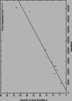
Figure 7 shows a plot of the processing times and the
corresponding number of instructions for each binary. The straight
line represents the linear regression line. The close proximity of all
points to this line demonstrates that the processing time
increases proportional to the number of instructions, allowing our
disassembler to operate on large binaries with acceptable
cost.
Figure 7:
Processing times and linear regression.
|
7 Conclusions
Correct disassembler output is crucial for many security tools such as
virus scanners [3] and intrusion detection
systems [11]. Recently, Linn and
Debray [13] presented obfuscation techniques that
successfully confuse current state-of-the-art disassemblers. We
developed and implemented a disassembler that can analyze obfuscated
binaries. Using the program's control flow graph and statistical
techniques, we are able to correctly identify a large fraction of the
program's instructions.
Obfuscation and de-obfuscation is an arms race. It is possible to
devise obfuscation techniques that will make the disassembly
algorithms describe in this paper less effective. However, this arms
race is usually in favor of the de-obfuscator. The obfuscator has to
devise techniques that transform the program without seriously
impacting the run-time performance or increasing the binary's size or
memory footprint while there are no such constraints for the
de-obfuscator. Also, the de-obfuscator has the advantage of going
second. That is, the obfuscator must resist all attacks, while the
de-obfuscator can tailor the attack to a specific obfuscation
technique. In this direction, a recent theoretical
paper [1] also proved that obfuscation is
impossible in the general case, at least for certain properties.
- 1
-
B. Barak, O. Goldreich, R. Impagliazzo, S. Rudich, A. Sahai, S. Vadhan, and
K. Yang.
On the (Im)possibility of Software Obfuscation.
In In Proceedings of Crypto, 2001.
- 2
-
J. Bergeron, M. Debbabi, M.M. Erhioui, and B. Ktari.
Static Analysis of Binary Code to Isolate Malicious Behaviors.
In In Proceedinsg of 8th IEEE International Workshops on
Enabling Technologies: Infrastructure for Collaborative Enterprises, 1999.
- 3
-
M. Christodorescu and Somesh Jha.
Static Analysis of Executables to Detect Malicious Patterns.
In Proceedings of the 12th USENIX Security Symposium, 2003.
- 4
-
C. Cifuentes and M. Van Emmerik.
UQBT: Adaptable binary translation at low cost.
IEEE Computer, 40(2-3), 2000.
- 5
-
C. Cifuentes and A. Fraboulet.
Intraprocedural Static Slicing of Binary Executables.
In Proceedings of the International Conference on Software
Maintenance (ICSM '97), Bari, Italy, October 1997.
- 6
-
C. Cifuentes and K. Gough.
Decompilation of Binary Programs.
Software Practice & Experience, 25(7):811-829, July 1995.
- 7
-
F. B. Cohen.
Operating System Protection through Program Evolution.
https://all.net/books/IP/evolve.html.
- 8
-
C. Collberg and C. Thomborson.
Watermarking, Tamper-Proofing, and Obfuscation - Tools for Software
Protection.
IEEE Transactions on Software Engineering, 28(8):735-746,
August 2002.
- 9
-
C. Collberg, C. Thomborson, and D. Low.
A Taxonomy of Obfuscating Transformations.
Technical Report 148, Department of Computer Science, University of
Auckland, July 1997.
- 10
-
Free Software Foundation.
GNU Binary Utilities, Mar 2002.
https://www.gnu.org/software/binutils/manual/.
- 11
-
J.T. Giffin, S. Jha, and B.P. Miller.
Detecting manipulated remote call streams.
In In Proceedings of 11th USENIX Security Symposium, 2002.
- 12
-
W.C. Hsieh, D. Engler, and G. Back.
Reverse-Engineering Instruction Encodings.
In Proceedings of the USENIX Annual Technical Conference, pages
133-146, Boston, Mass., June 2001.
- 13
-
C. Linn and S. Debray.
Obfuscation of executable code to improve resistance to static
disassembly.
In Proceedings of the 10th ACM Conference on Computer and
Communications Security (CCS), pages 290-299, Washington, DC, October 2003.
- 14
-
T. Ogiso, Y. Sakabe, M. Soshi, and A. Miyaji.
Software obfuscation on a theoretical basis and its implementation.
IEICE Transactions on Fundamentals, E86-A(1), 2003.
- 15
-
R. Sites, A. Chernoff, M. Kirk, M. Marks, and S. Robinson.
Binary Translation.
Digital Technical Journal, 4(4), 1992.
- 16
-
Symantec.
Understanding and Managing Polymorphic Viruses.
https://www.symantec.com/avcenter/whitepapers.html.
- 17
-
C. Wang, J. Davidson, J. Hill, and J. Knight.
Protection of Software-based Survivability Mechanisms.
In In Proceedings of International Conference of Dependable
Systems and Networks, 2001.
- 18
-
G. Wroblewski.
General Method of Program Code Obfuscation.
In Proceedings of the International Conference on Software
Engineering Research and Practice (SERP), Las Vegas, NV, June 2002.
Static Disassembly of Obfuscated Binaries
This document was generated using the
LaTeX2HTML translator Version 2002-2 (1.70)
Copyright © 1993, 1994, 1995, 1996,
Nikos Drakos,
Computer Based Learning Unit, University of Leeds.
Copyright © 1997, 1998, 1999,
Ross Moore,
Mathematics Department, Macquarie University, Sydney.
The command line arguments were:
latex2html -split 0 -show_section_numbers -local_icons disassemble.tex
The translation was initiated by on 2004-05-18
2004-05-18
|