Pp. 93–102 of the Proceedings

Preprocessor Algorithm for Network Management Codebook

Minaxi Gupta
College of Computing
Georgia Institute of Technology
801 Atlantic Drive, Atlanta, GA 30332-0280
minaxi@cc.gatech.edu

Mani Subramanian
Georgia Institute of Technology
manis@cc.gatech.edu

Abstract

As the size of networks increases, real-time fault management becomes difficult due to the volume of traffic. A single problem can generate numerous symptoms, which are received as events by a network management system. These events could be correlated to deduce the source of the problem. One of the correlation techniques used is codebook approach, developed by Yemini et. al. Codebook is a matrix relating problems with symptoms. We present a way to transform the original algorithm used in deriving the codebook. Our algorithm improves the efficiency by reducing the matrix as well as by ensuring the selection of minimum number of symptoms required to uniquely identify each problem in the codebook. This avoids an exponential growth in the number of symptoms as number of problems increase, which in turn shows up as saving in real-time processing.

Introduction

As the size of networks increases, real-time fault management becomes difficult due to the volume of traffic. A single problem can generate numberous symptoms, which are received as events by a network management system. These events could be correlated to deduce the source of the problem.

There are various fault correlation techniques available. Prominent ones out of these are: Rule-based reasoning (a rule base contains expert knowledge in the form of if-then or condition-action rules), Case-based reasoning (these systems store knowledge as a repository of successful cases of solved problems and when the system is presented with a problems, it searches for similar cases in its database), Reasoning with generic models (generic models rely on generic algorithms to correlate events based on an abstraction of system architecture and its components), Probability networks (these networks works on the probability of correctness of hypothesis about the state of the system), Model-based reasoning (this involves creating a model which represents the underlying system being monitored, an example of this would be a finite state machine), and codebook approach (this approach treats detection and identification of exception events in a system as a coding problem). Out of the above mentioned available event correlation and management approaches, we have selected Codebook Approach because of its superiority over the other techniques. The basic idea of this approach is to form a matrix relating potential problems with the symptoms that manifest them. Such a matrix is usually very large and for fast run-time detection, one needs to apply efficient algorithms to reduce its size (the resultant matrix is referred to as codebook, and is the main focus of this paper), still maintaining enough information to be able to detect and uniquely identify the root cause of the problem. Run-time decoding of problems uses the codebook and employs best-fit approaches to conclude the occurrence of problems.

The basis of our present work is the original work by Yemini et. al. ( [1, 2]) on codebook approach. In this paper, we present a method of pre-processing the matrix made up of problems and symptoms which produces optimal (minimal), mathematically provable codebook if the matrix lends itself to an optimal solution. The work presented in this paper improves upon the original codebook approach. The meaning of the terms used will be explained in more detail in subsequent sections.

Codebook Approach

In codebook approach ( [1, 2]), event correlation (correlating observed symptoms to specific problems) is split into two separate activities: (1) generating efficient codes for problem identification, and (2) decoding the event stream. Using this technique, detection and identification of problems in the system can be done efficiently due to following reasons. First, the redundant and inefficient data is eliminated during code generation, leaving a greatly reduced amount of data to be analyzed during the decoding phase, and second, comparing codes against observed symptoms significantly reduces computational complexity.

There is a four-step process that accomplishes the above. It includes

• Specifying an event model (possible problems that can occur in the system under consideration) and a propagation model (how these events propagate to generate observable symptoms) for components in the system. This specification includes the exceptional events associated with each type of component, their corresponding local symptoms, and the potential relationships with other components along which events can propagate.
• Creating a representation of possible problems and their symptoms for the system to be monitored. The preferred way for this type of representation is a matrix. This matrix contains a mapping of symptoms to likely problems in the system. Typically, such a matrix will contain 1s and 0s in each cell. Since some problems can occur with higher probability than other, probabilities can be included in this matrix to ensure more focus on problems that are more likely. By eliminating loops and repetitions of rows and columns, the matrix is made well-formed.
• Finding a minimal codebook by reducing the amount of information in the above matrix to the minimum required to identify uniquely problems. Codebook should be able to tolerate loss of events or generation of spurious symptoms, this can be done by introducing redundancy in the selected symptoms.
• Continuously monitoring and decoding the symptoms by locating the best-fit problem in the optimal codebook which matches a particular set of symptoms.

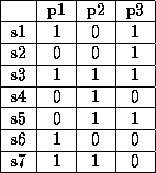
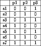
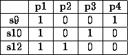
Optimal Codebook Generation

Our work assumes that first two stages of the codebook have been accomplished as described by Yemini et. al.  [2]. We start with a well-formed matrix. The goal is to reduce it to generate the optimal (minimal) codebook. Initially, we assume no error tolerance by our codebook. This means that loss of symptoms, or generation of spurious symptoms will result in incorrect decoding of problem occurrence at run-time.

To motivate the need for such a codebook, an example follows.

A well-formed matrix for a system with three problems represented by symptoms along rows and problems along columns is shown in Figure 1.

  
Figure 1: A well-formed matrix for three problem case

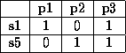
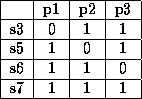
An optimal codebook, however, for above well-formed matrix would end up as in Figure 2.

  
Figure 2: Optimal codebook for matrix in Figure 1

As this simple example shows, only two symptoms are needed to distinguish among three problems, hence keeping seven symptoms (as the original well-formed matrix did) to be decoded at run-time is an overkill. In the subsequent discussion, we will explain the mathematical limits of the optimal number of symptoms that a codebook should have depending on the number of problems and how to achieve that limit.

Well-Formed Matrix

Ideally, a well-formed matrix for n problems should contain only symptoms at maximum. This is because, mathematically, there can be only combinations of 1s and 0s possible if there are no common rows. Out of these, the row containing all 0s does not help us distinguish any problems from each other(mathematically speaking, the row containing all 1s also does not help us distinguish any problem from any other, but in real world, that can be useful, hence we keep that), so those can be eliminated. We will assume that the well-formed matrix provided to us as input is an ideal one (that it has all possible combinations of 1s and 0s). This is what we mean by a matrix lending itself to optimal solution. A non-ideal matrix may be have far fewer rows to lend itself to optimal solution.

Mathematical Limits

Let's start with some motivation for what the algorithm should accomplish and what the mathematical limits are on the optimal codebook.

Given n problems, to be able to distinguish each problem from all others, we need following number of distinct cases

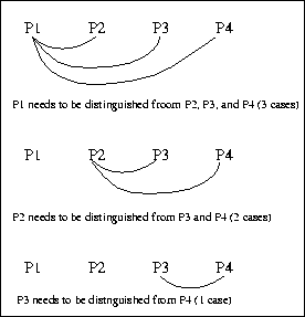
This is because the first problem needs to be distinguished from (n-1) other problems (hence, there are (n-1) cases), the second problem needs to be distinguished from (n-2) other problems (because the second problem has already been distinguished from the first) and so on. The (n-1)th problem just needs to be distinguished from 1 other problem, the last one. For a four problem case, the cases can be pictorially explained in Figure 3.

  
Figure 3: Enumeration of cases for four problem case

Total number of cases for four problem case: 3+2+1 = 6 If we substitute n=4 in Equation 1, we get the same result.

Each symptom eliminates several cases. If k symptoms are required to distinguish n problems, we want following to hold true:

The reason for this is as follows. If k symptoms are selected, we have combinations of 1s and 0s available at our disposal. Out of this, the combination consisting of all 0s needs to be ruled out, since that won't help distinguish any of the problems from any other.

There is a window of problems, that a certain number of symptoms can distinguish. This window (denoted by w) is given by

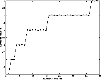
Figure 4 gives a feel for that window of problems. As is clear from the graph, the window keeps getting wider with n. The fact that these k symptoms are sufficient can be proven by checking that they have at least n(n-1)/2 cases embedded in them.

  
Figure 4: Windows of symptoms for various problem ranges

Pre-processing the Well-Formed Matrix

The pre-processing that we propose on the well-formed matrix is guided by the following observation. Intuitively, to select the minimum set of symptoms for the codebook, the best approach is to eliminate as many cases as possible with each symptom that we select. Let us now see how we can do that.

To distinguish n problems, if we select the first symptom of the type

1 0 0.... 0 (only one 1, rest (n-1) are 0s),

This would help us distinguish the first problem from all the other problems, but no other problems can be distinguished from any other problems. Hence it eliminates (n-1) cases out of the n(n-1)/2 that we need to eliminate. However, it is not the optimal one to select. Let us consider the case where we select a symptom that has approximately equal number of 1s and 0s (approximate, because for odd number of problems, number of 1s and 0s are not equal), i.e., the symptom was of the type

1 0 1 0 .... 1 0 (approximately n/2 0s and n/2 1s)

The 1s and 0s need not be in any specific order - we call such symptoms as balanced symptoms). This could eliminate 50% of the cases we need to eliminate right after the first symptoms is chosen (because of complementary nature of the symptom). Eliminating 50% would mean eliminating n(n-1)/4, which is larger than (n-1) for n>4 (implying larger the problems, better it is to start with balanced symptoms). The exact number of cases eliminated for each problem will depend on the particular combination of 1s and 0s in the balanced symptom.

For subsequent symptoms also, if we could eliminate as many rows as possible (upto 50%) of the remaining cases at each stage following similar procedure, we are guaranteed to select the minimum number of symptoms, because this would imply that we select approximately symptoms (this expression can be derived from Equation 2). We are now ready to detail pre-processing steps.

• Step 1: Sort the well-formed matrix, bring the balanced symptoms on top.
• Step 2: Eliminate compliments to prepare the matrix for our algorithm that selects codebook.

We would illustrate the effect of each step on sets of three and four problems.

Pre-Processing Algorithm

Step 1

We first sort the well formed matrix in our hand. We call this new matrix as sorted-well-formed matrix. The idea behind sorting is to keep the balanced symptoms on the top of the matrix (as explained in the previous section, balanced symptoms are the best ones to select). Figuring out whether a symptom is balanced or not takes O(n). This can be done in one pass and the time taken for this would be O(mn), where n is the number of problems and m is the number of symptoms. The next pass can naively go through this list of numbers and puts the balanced symptoms before the unbalanced ones (it will be a little more involved for matrices with odd number of problems, because for odd number of problems, rows with (n-1)/2 and (n+1)/2 1s in them will be balanced, as against the n/2 for even number of problems). The sort also takes time O( ), where m is the number of symptoms. There are many better algorithms that can be employed for this purpose, but since it does not affect the complexity of our solution, we would keep this simple one for the time being.

We now illustrate examples of sorting three (odd number of problems) and four (even number of problems) problem matrices.

A three problem well-formed matrix can have only seven combinations (of course many permutations of the rows are possible and the real world matrix may not even have all of them). Figure 5 shows a three problem well-formed matrix.

  
Figure 5: Another well-formed matrix for three problem case

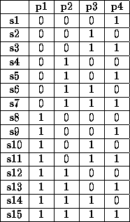
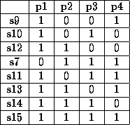
After sorting, it would not change for this particular case because all but the last combination of all 1's are balanced (except the last one).

For four problems, maximumwell-formed matrix would look like (fifteen combinations possible) Figure 6.

  
Figure 6: Well-formed matrix for four problem case

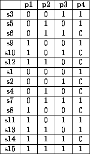
After sorting, the balanced symptoms get pushed to the top and the well formed matrix for four problems changes to give us Figure 7.

  
Figure 7: Sorted-well-formed matrix for four problem case

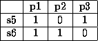
Step 2

Eliminate all the compliment rows from the well-formed matrix. If the matrix had all possible combinations in it, it would cut down the matrix size in half. The reason we eliminate the compliments is because although the compliments mean different symbols physically, they do not contain any different information from each other mathematically. To see that, consider symptoms in Figure 8.

  
Figure 8: Figure showing compliment symptoms

The first symptom distinguishes p1, p2 and p4 from p3. The same is the case with the second symptom.

While deciding to eliminate one of the compliments, we give preference to the symptom with more 1s in it. The reason for this choice is completely physical. The symptom with more 1s is likely to be more useful (because it shows up for more problems) than the one with more 0s. If there are equal number of 1s and 0s, we simply choose the one that has more 1s in the beginning. From the face of it, it seems more like a convention. But in reality, this helps select better symptoms. There can be other choices as well for choosing symptoms, logically, this seems to work the best.

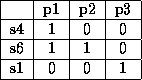
This operation takes O( ) time, where m is the number of symptoms because for every row, one may have to go all the way down to find the compliment and at each stage, O(n) comparisons are required for n problems.

After eliminating the compliments, while giving priority to the symptoms with more 1s than 0s, we get Figures 9, and 10 matrices for three and four problems respectively.

  
Figure 9: Minimized-sorted-well-formed matrix for three problems

  
Figure 10: Minimized-sorted-well-formed matrix for four problems

In the matrix for four problem case, s9 was given a priority over s6 while eliminating compliments because, although they have the same number of 1s and 0s in them, s9 has more 0s in the beginning than s6. Also, the matrix might look a little different depending on the exact algorithm that is used while re-shuffling the symptoms. We just mark the symptoms that we would eliminate and later just copy the un-marked ones in order.

These matrices are called minimized-sorted-well-formed matrices.

The number of balanced symptoms in the matrix for even and odd number of problems can be expressed by the formulae in Equations 4 and 5 respectively.

This is because for even number of problems, we just need to choose n/2 positions for 0s and 1s can go in the rest of the positions (and vice versa). For odd number of problems, there are two ways to choose balances symptoms. Hence correspondingly, for odd number of problems, there are two terms. Since we have eliminated compliments, the number of combinations that we get need to be halved, hence the above formulae. These formulae can be verified with the following results.

Codebook Algorithm

Having pre-processed the well-formed matrix, we will analyze the behavior of codebook algorithm using pre-processed matrix. Because of the pre-processing steps, the algorithm will always generate minimal codebook if the well-formed matrix contains adequate symptoms to uniquely distinguish between problems, i.e., it is always optimal.

The idea behind the algorithm is very simple. We start with the first problem and see how many symptoms will uniquely distinguish it from all other problems. For all other problems, we first check to see if the symptoms that have been already selected will suffice to distinguish it from all other problem. If the answer is yes, then we move on to the next problem, if not, then we determine which symptoms are to be added. We work our way through the input matrix sequentially.

We will illustrate the working of this algorithm on the minimized-sorted- well-formed matrix for three problems first.

• It chooses s5. s5 distinguishes p1 from p2 (s3 distinguishes p1 from p2, but does not show up for p1, while s5 shows up whenever p1 happens).
• To distinguish p1 from p3, the algorithm selects s6. Now p1 has been distinguished from all other problems.
• Now it will move on to other problems. In this case, it is just p2. The algorithm will first check to see if already selected symptoms are enough. It turns out that both s5 and s6 can be used to distinguish p2 from p3 as well. It should be noted that even s5 can be used to distinguish p2 from p3, though it does not show up for p2 (as explained later, a sanity check will eliminate the worst case scenario of running into a case where mathematically a problem can be diagnosed, but practically it can not be). Only when we pick a new symptom do we make sure that the symptom actually shows up for that particular problem.

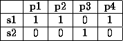
The algorithm selects two symptoms for three problems, which is the minimum required mathematically. The resulting codebook is shown in Figure 11.

  
Figure 11: Codebook for matrix of Figure 5

Running this algorithm on Figure 5 without pre-processing it, produces Figure 12.

  
Figure 12: Codebook for matrix of Figure 5, without pre-processing

This is not the optimal codebook because it has one more symptom than the minimum codebook. This shows that without pre-processing, optimal algorithm could fail to produce optimal codebook.

The algorithm will work on minimized-sorted well-formed matrix for four problems as follows.

• It chooses s9 because that is the first symptom that shows up for p1. s9 distinguishes p1 from p2 and p3.
• To distinguish p1 from p4, the algorithm will select s10 (the algorithm always starts from the first symptom). At this point, p1 has been distinguished from all other problems.
• For p2, s9 (which has already been selected), distinguishes it from p4 but not from p3 and s10 distinguishes it from p4. So, p2 is also taken care of.
• p3 can be distinguished from p4 using s9. So, all problems can be distinguished from each other.
• The algorithm does a sanity check at this stage (because it claims to have distinguished all problems in less symptoms than mathematically required). It turns out that if only s9 and s10 are used, even if p2 occurs, it would not show up. To avoid this, the algorithm selects s12 and is done generating the codebook at this time.

The resulting minimal codebook for four problem case would be as shown in Figure 13.

  
Figure 13: Codebook for matrix of Figure 6

It is clear that the algorithm selects three symptoms for four problems. It is easy to show that if the initial rows of the matrix are not made the right kind by pre-processing, because of the nature of the algorithm, it would selected many more symptoms (maximum number equal to the number of problems) than the optimal (hence the argument that the pre-processing work that we have done will eliminate the possibility of bigger codebooks). For small problem sets, this difference is not very prominent, but for larger problem sets, it could effect the run-time problem identification adversely. However, it should be noted that there could be some real-world matrices that will not have enough balanced symptoms (in particular, they may have lesser than the optimal codebook requirements). In that case, the algorithm will be forced to generate a sub-optimal codebook. In practice, the redundancy in the matrices is so much that such a case would be rare, else we will not really need codebooks at all!

Discussion

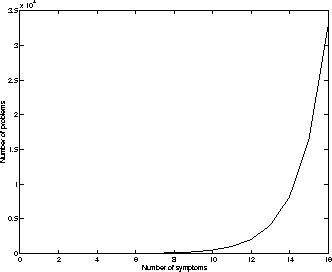
Figure 14 shows that the number of problems that can be detected at run-time by same number of symptoms increase exponentially. We have used the lower limit of the window of problems that can be detected using the same number of symptoms to be on the conservative side. We have used the relation (lower end of the window from Equation 3) as our y-axis parameter.

  
Figure 14: Number of problems that can be detected at run-time using same number of symptoms increase exponentially

We now compute net savings due to pre-processing input matrices.

At the higher end of a window (for example, n=15, k=4), savings are given by

At the lower end of the same window (n=8, k=4), savings are given by

Equations 6 and 7 give the reduction in the number of symptoms our preprocessor algorithm guarantees over worst case codebook (if the pre-processing of well-formed matrix was not done and codebook algorithm was run on it). The way we compute savings is as follows. Without pre-processing, in the worst case, for n problems, n symptoms will be selected by codebook algorithm to uniquely identify the problem. However, if the well-formed matrix is pre-processed, only or symptoms are needed for optimal codebook, depending on which end of the window one is in (these formulae are derived using Equation 3). Average number of symptoms required for a given number of problems are given by

Hence the average savings are given as

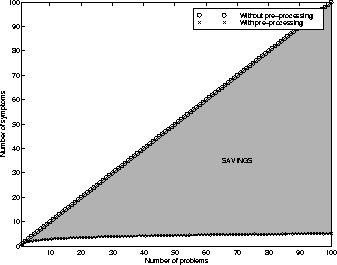
Figure 15 brings about some of these points more explicitly. It compares the number of symptoms in the final codebook generated using the codebook algorithm with and without the pre-processing of input matrix. As is very clear from the figure, pre-processing reduces the number of symptoms substantially. Also, as the number of problems increases, the savings increase, making the difference more prominent (and in turn, ensuring more real-time savings).

  
Figure 15: Comparison of number of symptoms in output codebook with and without pre-processing of input matrix

Summary

We have developed a two step pre-processing algorithm that ensures that the codebook algorithm would generate mathematically provable optimal codebook. Using the pre-processing algorithm for a given number of symptoms, number of problems that can be identified increases exponentially. For a practical situation, number of problem being finite, number of symptoms needed reaches a plateau, if the pre-processing algorithm is used.

References

1

United States Patent. Apparatus and method for event correlation and problem reporting. Yemini et al. Jun-18-1996.

2

High speed and robust event correlation. Yemini et al. May-1996.

About this document ...

Preprocessor Algorithm for Network Management Codebook

This document was generated using the LaTeX2HTML translator Version 96.1-e (April 9, 1996) Copyright © 1993, 1994, 1995, 1996, Nikos Drakos, Computer Based Learning Unit, University of Leeds.

The command line arguments were:
latex2html -split 0 report.tex.

The translation was initiated by Minaxi Gupta on Mon Feb 22 16:32:21 EST 1999