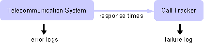
Figure 2:
Experimental setup. Call response times have
been tracked from outside the system in order to identify failures.
We had access to data collected at 200
non-consecutive days spanning a
period of 273 days. The entire dataset consists of error logs with a
total of 26,991,314 log records including 1,560 failures of two types:
The first type (885 instances) relates to GPRS and the second (675
instances) to SMS and MOC services. In this study, only the first
failure type has been investigated.
3 Data
Preprocessing
3.1 Creating
Machine Processable Logfiles
Traditionally, logfiles
were intended to be read by humans in order to
support fault diagnosis and root cause analysis after a system had
failed. They are not well-suited for machine processing. An
(anonymized) example log record consisting of three lines in the error
log is shown in Figure
3.
2004/04/09-19:26:13.634089-29846-00010-LIB_ABC_USER-AGOMP#020200034000060|020101044430000|000000000000-020234f43301e000-2.0.1|020200003200060
2004/04/09-19:26:13.634089-29846-00010-LIB_ABC_USER-NOT:
src=ERROR_APPLICATION sev=SEVERITY_MINOR id=020d02222083730a
2004/04/09-19:26:13.634089-29846-00010-LIB_ABC_USER-unknown nature of
address value specified
Figure 3:
Anonymized error log record from the
telecommunication system. The record consists of three log lines.
In order to simplify
machine processing, we applied the transformations
described in the following paragraphs.
Eliminating
logfile rotation.
Logfile rotation denotes a technique to switch to a new logfile when
the current logfile has reached a size limit, time span limit, or both.
In the telecommunication system logging was organized in a ring-buffer
fashion consisting of n logfiles. Data has been
reorganized to form one large chronologically ordered logfile.
Identifying
borders between messages.
While error messages "travel" through various modules and architectural
levels of the system, more and more information is accumulated until
the resulting log-record is written to the logfile. This often leads to
situations where the original error message is quoted several times
within one log record and one log record spans several lines in the
file. We eliminated duplicated information and assigned each piece to a
fixed column in the log such that each line corresponds to exactly one
log record. This also involved the usage of a unique field delimiter.
Converting
time. Timestamps in
the original logfiles were tailored to humans and had the form 2004/04/09-19:26:13.634089
stating that the log message occurred at 7:26pm and 13.634089 seconds
on 04/09/2004. In order to enable, e.g., computation of the time
interval between two error messages we transformed each timestamp into
real-valued UTC, which roughly relates to seconds since
Jan. 1st, 1970. This also involved the issue of timezone
information.
3.2 Assigning
IDs to Error Messages
Many error analysis tools
including the HSMM failure predictor rely on
an integer number to characterize the type of each error message.
However, in our case such an identifier was not available. This section
describes the algorithm we used to assign an ID to each error message
in the log.
The type of an error report
is only implicitly given by a natural
language sentence describing the event. In this section, we propose a
method to automatically assign error IDs to messages on the basis of
Levenshtein's edit distance. Note that the error ID is meant to
characterize
what has happened, which corresponds
to the
type of an error message in contrast to
the message
source, as has been discussed in
[6].
Removal of
numbers.
Assume that the following message occurs in the error log
process 1534: end of buffer reached
The situation that exactly
process with number 1534 reaches the end of
a buffer will occur rather rarely. Furthermore, the process number
relates to the source rather than the type of the message. Hence, all
numbers and log-record specific data such as IP addresses, etc. are
replaced by placeholders. For example, the message shown above is
translated into:
process xx: end of buffer reached
In order not to loose the
information, a copy of the original message
is kept.
Number
assignment. Since a 100%
complete replacement of all record-specific data is infeasible (there
were even typos in the error messages) error IDs are assigned on the
basis of Levenshtein's edit distance [
7] expressing
dissimilarity of messages. After number removal, Levenshtein distance
is computed between all pairs of log messages appearing in the log. By
applying a threshold on dissimilarity, similar messages receive the
same integer number - the error ID.
Applying this algorithm to
the telecommunication data resulted in an
immense reduction of the number of message types: While in the original
dataset there were 1,695,160 different log-messages, the number of
message types could be reduced to 1,435 (see Table
1)
| Data |
No of msgs |
Reduction in % |
| Original |
1,695,160 |
n/a |
| Without numbers |
12,533 |
99.26% |
| Levenshtein |
1,435 |
88.55% / 99.92% |
Table 1:
Number of different log messages in the original
data, after substitution of numbers by placeholders, and after
clustering by the Levenshtein distance metric.
Applying a simple threshold
might seem too simplistic to make a
decision which messages are grouped together. However, experiments have
shown that this is not the case. Figure
4 provides a
plot where the gray value of each point indicates Levenshtein distance
of the corresponding message pair for a selection of messages. In the
plot all messages that are assigned the same error ID are arranged next
to each other. Except for a few blocks in the middle of the plot, dark
steps only occur along the main descending diagonal and the rest of the
plot is rather light-colored. This indicates that strong similarity is
only present among messages with the same ID and not between other
message types. In addition to the plot, we have manually checked a
selection of a few tens of messages. Hence using a fixed threshold is a
simple yet robust approach. Nevertheless, as is the case for any
grouping algorithm it may assign the same ID to two error message that
should be kept separate. For example, if process 1534 was a crucial
singleton process in the system (like the "init" process in the Linux
kernel, which always has process ID one) the number would be an
important piece of information that should not be eliminated. However,
in our case the significant reduction in the number of messages
outweighs such effects. Note that Levenshtein distances have to be
computed only once for any pair of messages.

Figure
4: Levenshtein similarity plot for a subset of message
types. Points represent Levenshtein distance between one pair of error
messages (dark color indicates small distance).
3.3 Tupling
In
[8],
the authors note that repetitive log records occurring more or less at
the same time are frequently multiple reports of the same fault. Tsao
and Siewiorek introduced a procedure called
tupling,
which basically refers to grouping of error events that occur within
some time interval or that refer to the same location
[9].
Current research aims at quantifying temporal and spatial tupling. For
example, in
[10] the authors
introduce a correlation measure for this purpose.
We adopt the tupling method
of
[9].
However, equating the
location reported in an error message with the true location of the
fault only works for systems with strong fault containment regions.
Since this assumption does not hold for the telecommunication system
under consideration, spatial tupling is not considered any further,
here. The basic idea of tupling is that all errors showing an
inter-arrival time less than a threshold

are grouped.
1
Grouping can lead to two problems:
-
Error messages might
be combined that refer to several
(unrelated) faults. This is called a collision.
-
If an inter-arrival
time >
occurs within the error pattern of one single fault, this pattern is
divided into more than one tuple. This effect is called
truncation.
Both the number of
collisions and truncations depend on
.
If
is large, truncation happens rarely and collision will occur very
likely. If
is small
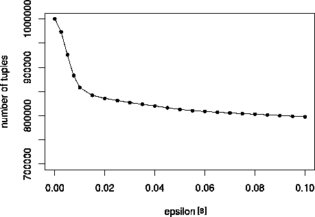
the effect is vice versa. To find an optimal
,
the authors suggest to plot the number of tuples over
.
This should yield an L-shaped
curve: If
equals zero,
the number of tuples equals the number of error events in the logfile.
While
is increased,
the number drops quickly. When the optimal value for
is reached, the curve flattens
suddenly. Our data supports this claim: Figure
5 shows the
plot for a subset of one million log records. The graph shows a clear
change point and a value of
= 0.015
s has been chosen.
3.4 Extracting
Sequences
Two types of data sets are
needed to train the HSMM-based failure
predictor: a set of failure-related error sequences and a set of
non-failure-related sequences. In order to decide whether a sequence is
a failure sequence or not, the failure log, which has been written by
the call tracker, has been analyzed, to extract timestamps and types of
failure occurrences.
In this last step of data preprocessing both types of sequences are
extracted from the data set.
Three parameters are
involved in sequence extraction:
-
Lead-time.
In order to predict
failures before a failure occurs, extracted failure sequences preceded
the time of failure occurrence by time
 tl
tl.
In the experiments we used a value of five minutes.
-
Data window
size. The length of each
sequence is determined by a maximum time
td.
In the experiments we used sequences of five minute length.
-
Margins for
non-failure sequences.
The set of non-failure sequences should be extracted from the log at
times when the system is fault-free. However, whether a system really
is fault-free is hard to tell. Therefore, we applied a "ban period" of
size
tm
before and after a failure. By visual inspection (length of bursts of
failures, etc.), we determined
tm
to be 20 minutes.
Non-failure sequences have
been generated using overlapping time
windows, which simulates the case that failure prediction is performed
each time an error occurs, and a random selection has been used to
reduce the size of the training data set.
4 Failure
Sequence Clustering
The term
failure
mechanism, as used in this
paper, denotes a principle chain of actions or conditions that leads to
a system failure. It is assumed that in complex computer systems such
as the telecommunication system various failure mechanisms can lead to
the same failure. Different failure mechanisms can show completely
different behavior in the error event logs, which makes it very
difficult for the learning algorithm to extract the inherent
"principle" of failure behavior in a given training data set. The idea
of clustering failure-related error sequences (which for brevity
reasons from now on will be called "failure sequences") is to group
similar sequences and train a separate HSMM for each group. Failure
sequence clustering aims at grouping failure sequences according to
their similarity - however, there is no "natural" distance metric such
as Euclidean norm for error event sequences. We use sequence
likelihoods from small HSMMs for this purpose. The approach is inspired
by
[11]
but yields separate specialized models instead of one mixture model.
4.1 Obtaining
the Dissimilarity Matrix
Most clustering algorithms
require as their input data a matrix of
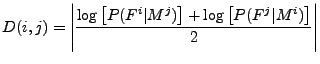
dissimilarities among data points (D). In our case,
each data point is a failure sequence Fi
and hence D(i,j)
denotes the dissimilarity between failure sequence Fi
and Fj.
As first step a small HSMM Mi
is trained separately for each failure sequence Fi.
The objective of the training algorithm is to adjust the HSMM
parameters (e.g., transition probabilities and observation probability
distributions) to the training sequence, i.e., the HSMM is tuned such
that it assigns a high sequence likelihood to the training sequence.
In order to compute
D(
i,
j)
the sequence likelihood
P(
Fi
| Mj)
is computed for each sequence
Fi
using each model
Mj.
Sequence likelihood is used as a similarity score

[0,1]. Since model
Mj
has been trained with sequence
Fj,
it assigns a high sequence likelihood to sequences
Fi
that are similar to
Fj,
and a lower sequence likelihood to sequences
Fi
that are less similar to
Fj.
In order to avoid numeric instabilities, the logarithm of the
likelihood (log-likelihood) is used (see Figure
6).
The resulting matrix is not
yet a dissimilarity matrix, since first,
values are

0
and second, sequence likelihoods are not symmetric:
P(
Fi
| Mj)
 P
P(
Fj
| Mi).
This is solved by taking the arithmetic mean of both likelihoods and
using the absolute value. Hence
D(
i,
j)
is defined as:
Still, matrix
D
is not a proper dissimilarity
matrix since a proper metric requires that
D(
i,
j)
= 0, if
Fi
=
Fj.
There is no solution to this problem since from
D(
j,
j)
= 0 follows that
P(
Fj
| Mj)
= 1. However, if
Mj
would assign a probability of one to
Fj
it would assign a probability of zero to all other sequences
Fi
Fj,
which would be useless for clustering. Nevertheless,
D(
j,
j)
is close to zero since it denotes log-sequence likelihood for the
sequence, model
Mj
has been trained with.
In order to achieve a good
measure of similarity among sequences models
should not be overfitted to their training sequences. Furthermore, one
model needs to be trained for each failure sequence in the training
data set. Therefore, models
Mi
have only a few states and are ergodic (have the structure of a
clique). An example is shown in Figure
7. In order to further
avoid too specific models, exponential distributions for inter-error
durations and a uniform background distribution have been used.
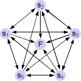
Figure 7:
Topology of HSMMs used for computation of the
dissimilarity matrix. Observation symbol probabilities are omitted.
Background distributions
add some small probability to all HMM
observation probabilities following a (data independent) distribution
such as uniform.
4.2 Grouping
Failure Sequences
In order to group similar
failure sequences, a clustering algorithm has
been applied to the dissimilarity matrix. Due to the fact that the
number of groups cannot be determined upfront and can vary greatly, we
applied hierarchical clustering methods (both agglomerative and
divisive, c.f., e.g.,
[12]). The actual
number of groups has been determined by visual inspection of banner
plots.
4.3 Analysis
of Sequence Clustering
The failure sequence
clustering approach implies several parameters
such as the number of states of the HSMMs, or the clustering method
used. This section explores their influence on sequence clustering (not
on failure prediction accuracy, which is investigated in
Section
6). In
order to do so many combinations of parameters have been analyzed, but
only key results can be presented here. In order to support clarity of
the plots, a data excerpt from five successive days including 40
failure sequences has been used.
We explored one divisive
algorithm (DIANA), and four agglomerative
approaches (AGNES) using single linkage, average linkage, complete
linkage and Ward's procedure (c.f.
[12]) Figure
8 shows banner
plots for all methods using a dissimilarity matrix that has been
generated using a HSMM with 20 states and a uniform background
distribution with a weighting factor of 0.25. Banner plots connect data
points (sequences) by a bar of length to the level of distance metric
where the two points are merged / divided.
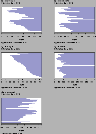
Figure 8:
Clustering of 40 failure sequences using five
different clustering methods: agglomerative clustering ("agnes") using
average, complete, and single linkage, agglomerative clustering using
Ward's method and divisive clustering ("diana").
Single linkage clustering
(second row, left) shows the typical chaining
effect, which does not result in a good separation of failure sequences
yielding an agglomerative coefficient of only 0.45. Complete linkage
(first row, right) performs better resulting in a clear separation of
two groups and an agglomerative coefficient of 0.72. Not surprisingly,
average linkage (first row, left) resembles some mixture of single and
complete linkage clustering. Divisive clustering (bottom row, left)
divides data into three groups at the beginning but does not look
consistent since groups are split up further rather quickly. The
resulting agglomerative coefficient is 0.69. Finally, agglomerative
clustering using Ward's method (second row, right) results in the
clearest separation achieving an agglomerative coefficient of 0.85. The
results are roughly the same if other parameter settings are
considered.
In order to investigate the
impact of the number of states
N
of the HSMMs, we performed several experiments ranging from five to 50
states. We found that failure grouping only works well if the number of
states is roughly above

where
L denotes the average length of the
sequences. This might be explained by the fact that there are roughly
N2
transitions in the model.
We also investigated the
effect of background distributions and found
that some background distribution is necessary (otherwise, each model
only recognizes exactly the sequence it has been trained with).
However, the actual strength (or weight) of the background distribution
has only small impact as long as it stays in a reasonable range (if the
weighting factor for background distributions gets too large, the
"chaining-effect" can be observed and the agglomerative coefficient is
decreasing).
5 Filtering
the Noise
The objective of the
previous clustering step was to group failure
sequences that are traces of the same failure mechanism. Hence it can
be expected that failure sequences of one group are more or less
similar. However, experiments have shown that this is not always the
case. The reason for this is that error logfiles contain noise
(unrelated events), which results mainly from parallelism within the
system. Hence we applied some filtering to eliminate noise and to mine
the events in the sequences that make up the true pattern.
The filtering mechanism is
based on the notion that within a certain
time window prior to failure, indicative events occur more frequently
within failure sequences of the same failure mechanism than within all
other sequences. The precise definition of "more frequently" is based
on the

test of goodness of fit.
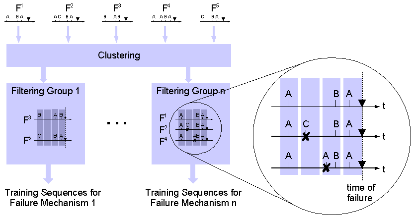
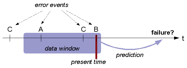
Figure 9:
After clustering similar failure sequences,
filtering is applied to remove failure unrelated errors from training
sequences. Times of failure occurrence are indicated by .
The filtering process is
depicted in the blow-up of Figure
9
and performs the following steps:
-
Prior probabilities
are estimated for each symbol. Priors
express the "general" probability that a given symbol occurs.
-
All failure sequences
of one group (which are similar and
are expected to represent one failure mechanism), are aligned such that
the failure occurs at time t=0. In the figure,
sequences F1, F2,
and F4 are aligned and the
dashed line indicates time of failure occurrence.
-
Time windows are
defined that reach backwards in time. The
length of the time window is fixed and time windows may overlap. Time
windows are indicated by shaded vertical bars in the figure.
-
The test is performed
for each time window separately,
taking into account all error events that have occurred within the time
window in all failure sequences of the group.
-
Only error events that
occur significantly more frequently
in the time window than their prior probability stay in the set of
training sequences. All other error events within the time window are
removed.
-
Filtering rules are
stored for each time window specifying
error symbols that pass the filter. The filter rules are used later for
online failure prediction in order to filter new sequences that occur
during runtime.
More formally, each error
ei
that occurs in failure sequences of the same cluster within a time
window (
t-t,
t]
prior to failure is checked for significant deviation from the
prior

by a test variable known from

-grams,
which are a non-squared version of the testing variable of the
goodness of fit test (see, e.g.,
[13]). The
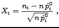
testing variable
Xi
is defined as the non-squared standardized difference:
where ni
denotes the number of occurrences of error ei
and n is the total number of errors in the time
window. An analysis reveals that all Xi
have an expected value of zero and variance of one, hence
they can all be compared to one threshold c:
Filtering eliminates all errors ei
from the sequences within the time window, for which Xi
< c. For online prediction, the sequence
under investigation is filtered the same way before sequence likelihood
is computed.
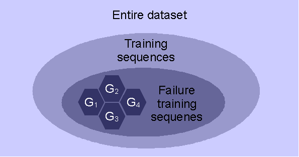
Figure 10:
The three different sequence sets that can be
used to compute symbol prior probabilities.
Three variants regarding
the computation of priors
exist (see Figure
10):
-
are
estimated from all training sequences (failure and non-failure).
Xi
compares the frequency of occurrence of error
ei
to the frequency of occurrence within the entire training data.
-
are estimated from all
failure
sequences
(irrespective of the groups obtained from clustering).
Xi
compares the frequency of occurrence of error
ei
to all failure sequences (irrespective of the group).
-
are estimated separately for each
group of failure sequences from all
errors within the group (over all time windows). For each error
ei
the testing variable
Xicompares the occurrence
within one time window to the entire group of
failure sequences.
Experiments have been
performed on the dataset used previously for
clustering analysis and six non-overlapping filtering time windows of
length 50 seconds have been analyzed. Figure
11
plots the average number of symbols in one group of failure sequences
after filtering out all errors with
Xi
<
c for various values of
c.
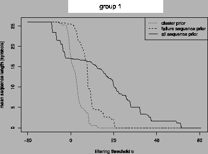
Figure 11:
Mean sequence length depending on threshold c
for three different priors.
Regarding the prior
computed from all sequences (solid line), all
symbols pass the filter for very small thresholds. At some value of
c
the length of sequences starts dropping quickly until some point where
sequence lengths stabilize for some range of
c.
With further increasing
c average sequence length
drops again until finally not a single symbol passes filtering. Similar
to the tupling heuristic by
[8], we consider a
threshold at he beginning of the middle plateau to best distinguish
between "signal" and noise. Other priors do not show this behavior,
hence we used priors estimated from all sequences (first prior).
6 Results
As stated before, the
overall objective was to predict failures of the
telecommunication system as accurate as possible. The metric used to
measure accuracy of predictions is the so-called
F-measure,
which is the harmonic mean of precision and recall.
Precision
is the relative number of correctly predicted failures to the total
number of predictions, and
recall is the relative
number of correctly predicted failures to the total number of failures.
A definition and comprehensive analysis can be found in
Chapter 8.2 of
[5]. The HSMM
prediction method involves a customizable threshold determining whether
a failure warning is issued very easily (at a low level of confidence
in the prediction) or only if it is rather sure that a failure is
imminent, which affects the trade-off between precision and recall.
2
In this paper we only report maximum achievable F-measure.
Applying the full chain of
data preparation as described in
Sections
3
to
5 yields a
failure prediction F-measure of 0.66. A comparative study has shown
that this result is significantly more accurate than best-known
error-based prediction approaches (see Chapter 9.9 of
[5]).
In order to determine the effect of clustering and filtering, we have
conducted experiments based on ungrouped (unclustered) data as well as
on unfiltered data. Unfortunately, experiments with neither filtering
nor grouping were not feasible. All experiments have been performed
with the same HSMM setup (i.e., number of states, model topology,
etc.). Results unveil that data preparation plays a significant role in
achieving accurate failure predictions (see Table
2).
| Method |
Max. F-Measure
|
rel. Quality |
| Optimal results |
0.66 |
100% |
| Without grouping |
0.5097 |
77% |
| Without filtering |
0.3601 |
55% |
Table 2:
Failure prediction accuracy expressed as maximum
F-measure from data with full data preparation, without failure
sequence grouping (clustering) and without noise filtering.
7 Conclusions
It is common perception
today that logfiles, and in particular error
logs, are a fruitful source of information both for analysis after
failure and for proactive fault handling which frequently builds on the
anticipation of upcoming failures. However, in order to get (machine)
access to the information contained in logs, the data needs to be put
into shape and valuable pieces of information need to be picked from
the vast amount of data. This paper described the process we used to
prepare error logs of a commercial telecommunication system for a
hidden semi-Markov failure predictor.
The preparation process
consists of three major steps and involved the
following new concepts: (a) an algorithm to automatically assign
integer error IDs to error messages, (b) a clustering algorithm for
error sequences, and (c) a statistical filtering algorithm to reduce
noise in the sequences. We conducted experiments to assess the effect
of sequence clustering and noise filtering. The results unveiled that
elaborate data preparation is a very important step to achieve good
prediction accuracy.
In addition to failure
prediction the proposed techniques might also be
helpful to speed up the process of diagnosis: For example, if root
causes have been identified for each failure group in a reference data
set, identification of the most similar reference sequence would allow
a first assignment of potential root causes for a failure that has
occurred during runtime.
References
- [1]
- R. K. Iyer, L. T. Young, and
V. Sridhar. Recognition of error symptoms in large systems. In
Proceedings of 1986 ACM Fall joint computer conference,
pages 797-806, Los Alamitos, CA, USA, 1986. IEEE Computer Society
Press.
-
- [2]
- Paul Horn. Autonomic computing: IBM's perspective on the
state of information technology, Oct. 2001.
-
- [3]
- Adam Oliner and Jon Stearley. What supercomputers say: A
study of five system logs. In IEEE proceedings of
International Conference on Dependable Systems and Networks (DSN'07),
pages 575-584. IEEE Computer Society, 2007.
-
- [4]
- David Bridgewater. Standardize messages with the common
base event model, 2004.
-
- [5]
- Felix Salfner. Event-based Failure Prediction:
An Extended Hidden Markov Model Approach. dissertation.de -
Verlag im Internet GmbH, Berlin, Germany, 2008. (Available as PDF).
-
- [6]
- Felix Salfner, Steffen Tschirpke, and Miroslaw Malek.
Comprehensive logfiles for autonomic systems. In IEEE
Proceedings of IPDPS, Workshop on Fault-Tolerant Parallel, Distributed
and Network-Centric Systems (FTPDS), 2004.
-
- [7]
- Alberto E. D.T. Apostolico and Zvi Galil. Pattern
Matching Algorithms. Oxford University Press, 1997.
-
- [8]
- R. Iyer and D. Rosetti. A statistical
load dependency of cpu errors at slac. In IEEE Proceedings
of 12th International Symposium on Fault Tolerant Computing (FTCS-12),
1982.
-
- [9]
- M. M. Tsao and Daniel P. Siewiorek. Trend
analysis on system error files. In Proc. 13th International
Symposium on Fault-Tolerant Computing, pages 116-119,
Milano, Italy, 1983.
-
- [10]
- Song Fu and Cheng-Zhong Xu. Quantifying temporal and
spatial fault event correlation for proactive failure management. In IEEE
Proceedings of Symposium on Reliable and Distributed Systems (SRDS 07),
2007.
-
- [11]
- Padhraic Smyth. Clustering sequences with hidden Markov
models. In Michael C. Mozer, Michael I. Jordan, and
Thomas Petsche, editors, Advances in Neural Information
Processing Systems, volume 9, page 648. The MIT
Press, 1997.
-
- [12]
- Leonard Kaufman and Peter J. Rousseeuw. Finding
Groups in Data. John Wiley and Sons, New York, 1990.
-
- [13]
- Rainer Schlittgen. Einführung in die
Statistik: Analyse und Modellierung von Daten.
Oldenbourg-Wissenschaftsverlag, München, Wien, 9 edition, 2000.
Footnotes:
1In
[9],
there is a second, larger threshold to add later events if they are
similar, but this is not considered, here
2In
fact, either precision or recall can be increased to 100% at the cost
of the other.