|
USENIX 2003 Annual Technical Conference, FREENIX Track — Paper
[USENIX Annual Conference '03 Tech Program Index]
| Pp. 63-76 of the Proceedings | |
Learning Spam: Simple Techniques
For Freely-Available Software
Bart Massey Mick Thomure
Raya Budrevich Scott Long
Computer Science Department
Portland State University
Portland, OR USA
bart,thomure,binargrl,scottl@cs.pdx.edu
https://oss.cs.pdx.edu/psam
The problem of automatically filtering out spam e-mail
using a classifier based on machine learning methods is of
great recent interest. This paper gives an introduction
to machine learning methods for spam filtering, reviewing
some of the relevant ideas and work in the open source
community. An overview of several feature detection and
machine learning techniques for spam filtering is given.
The authors' freely-available implementations of these
techniques are discussed. The techniques' performance on
several different corpora are evaluated. Finally, some
conclusions are drawn about the state of the art and about
fruitful directions for spam filtering for
freely-available UNIX software practitioners.
There has been a great deal of interest of late in the
problem of automatically detecting and filtering out
unsolicited commercial e-mail messages, commonly referred
to as spam. (While the Hormel Corporation, owners of
the ``Spam'' trademark, are not happy about the choice of
name, they have acceded to the popular usage. For a
further etymology see [14].) Recent
dramatic increases in spam volume have combined with the
success of a number of new filtering methods to make
automated spam filtering highly successful. The
SpamAssassin [20] mail-filtering tool is
one such tool. SpamAssassin uses a large
manually-generated feature set and a simple perceptron
classifier with hand-tuned weights to select ham
(non-spam) messages and discard spam.
Much current interest has focused around the role of machine learning [5,15] in
spam filtering methodologies. This paper describes the
basics of machine learning and several simple supervised
machine-learning algorithms that are effective in
filtering spam. The authors have made implementations of
these algorithms publically available, along with various
kinds of feature data from several corpora used to
evaluate the algorithms. These implementations and data
are used to help evaluate the relative merits of these
algorithms, and suggest directions for future work.
The spam problem has received increasing attention in
recent years. As a result, a number of approaches for
dealing with the problem have been proposed. A recent
issue of Wired magazine [11] lists a variety
of popular strategies. Blacklists such as
spamcop.net attempt to stop spam by preventing
spam-delivering hosts from communicating with the rest of
the Internet, or at least with the victim machine. Distributed identification systems such as Vipul's Razor
allow users to manually identify spam for collaborative
filtering. Header analysis can be used to eliminate
messages that have malformed or unusual headers or header
fields, as well as messages that have invalid return
addresses or sender information. Legal approaches
are gaining currency at both the U.S. State and Federal
levels, including proposed penalties for unsolicited
commercial e-mail and anonymous commercial messages. (It
should be noted that the legal approach is widely credited
with largely eliminating unsolicited commercial messages
via FAX.) The range of approaches is growing rapidly in
response to the increase in spam traffic: approaches not
noted by Wired include whitelist systems such as
Active Spam Killer [16], a mailback system
that attempts to verify that e-mail is ham by
requiring a confirmation message from unknown senders.
A recent conference on the spam problem at
MIT [8] was nearly overwhelmed by
the volume of attendees. The presentations
were quite productive; many critical points
were raised about spam filtering that deserve wider
attention by the open source community.
There was far too much useful information to
summarize here: perhaps one example will suffice.
There seems to be a widespread
perception that false positives (ham messages flagged as
spam by filters) are ``intolerable'' in spam filtering.
The MIT Spam Conference presenters mentioned several
reasons why insisting on zero tolerance for false
positives can lead users to wrongly reject spam filtering
as a technology. As many researchers have noted,
the absolute prohibition of false positives can only be
justified by assuming that they have infinite cost: while
a false positive may have a cost much larger than a false
negative [10], this cost is not
infinite. Further, false positive rates of most filtering
algorithms can be lowered in a tradeoff for false negative
rates. Finally, a good spam filter may actually exhibit
super-human classification performance: after all, this is
the sort of repetitive and error-prone task that a human
may be expected to perform
poorly [12]. The unsophisticated
filters reported here uniformly achieve false positive
rates of just a few percent: the authors informally
estimate their human false positive rates to be in a
similar range. Third, the false positive rate of a single
spam filter is somewhat irrelevant: both ensembles of
filters and the combination of filtering with other
approaches to spam detection can largely take care of the
overall false positive problem. Finally, spam will only
be sent if it is profitable: in the long haul, widespread
use of filters may change the economics of spamming enough
to largely eliminate the problem [7].
Research in spam filtering within the freely available
software community is currently proceeding quite quickly:
some of what is said here about the state of the art will
no longer be true by the time it is published.
The general system engineering and machine learning
principles that are key to the spam elimination effort,
however, should still be valuable for some time.
3 Machine Learning
Machine learning is a field with a broad and deep history.
In general, a machine learner is a program or device that
modifies current behavior by taking into account
remembered past results. This is a broad definition.
However, much of machine learning research is focused on
inductive learning, in which general rules are built
based on a corpus, a set of specific examples. In
spam filtering (and many other applications) the corpus
consists of pre-classified examples, and the learned
rules are used to classify e-mail as either ham or
spam.
This paper gives greatest emphasis to supervised
learning. In supervised learning, the examples to be used
for learning are collected and processed during a training phase. The learned rules are then used without
further modification during a classification phase.
Reinforcement learning--on-line correction of the
learned rules in response to classification errors--is
also quite valuable. This allows the system to adapt to
changing conditions, such as user preferences or spam
content. The simplistic approach of re-learning the
entire corpus, including newly acquired classifications, can
suffice if the learner is sufficiently fast on large
inputs.
Supervised machine learning for spam classification begins
with a corpus consisting of a collection of correctly
classified ham and spam messages. In the feature
selection stage, key features of the corpus are
identified that distinguish ham from spam. In
the training stage, the selected features of the corpus
are studied to learn characteristics that differentiate
spam from ham messages. Concurrently or subsequently, a
validation stage is often used to check the accuracy
of the learned characteristics. Finally, the learned
knowledge is used in a classification stage that filters
spam by giving a classification to each target
message in the classification set.
Some important considerations in supervised learning
involve management of the corpus. For accuracy's sake,
one would like to use the entire corpus as training data.
Unfortunately, this makes validation quite difficult:
the classifier will appear to perform unrealistically
well when asked to classify the messages on which it was trained.
Fortunately, in most problem domains the
number of training instances needed to learn with a given
accuracy grows only logarithmically with the size of the
hypothesis space, the set of concepts that must be
distinguished. Thus, it is customary to split the corpus
into a training set and a validation set. A
rule of thumb in machine learning is to make the
validation set consist of a randomly selected third of the
corpus. There are much more sophisticated methods
for validation that improve on the quality of this
approach, but the simple method will suffice for most cases.
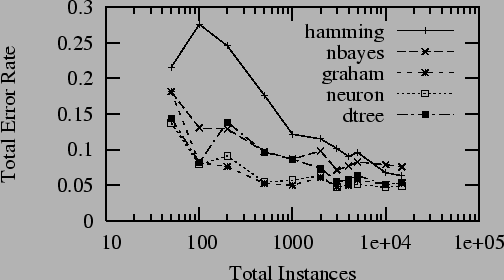
It is reasonable to be concerned about the minimum corpus
size required for full accuracy. As corpus size
increases, machine learning algorithms tend to asymptotically
approach their maximum accuracy. Figure 1
shows the accuracy of a number of different machine learning
algorithms on increasingly large subsets of a synthetic
corpus discussed in Section 7. The figure
shows that for the algorithms discussed here, 100-1000
messages are sufficient to achieve maximal accuracy. The
variance at low corpus sizes is due to statistical error,
and represents a large inter-run variance.
Figure 1:
Learning Rate
 |
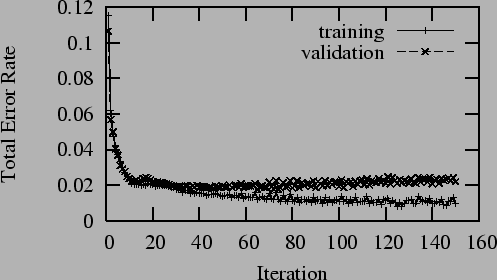
A risk that must be countered when training a machine
learner is overtraining: building a learner that
classifies based on quirks of the training set rather
than general properties of the corpus.
Figure 2 shows the change
in classification rate during training for the
perceptron of Section 4.2.4 on the
15,000 instance personal e-mail corpus described in
Section 7. In the figure, the accuracy of
classification on the training set continues to increase,
while the accuracy on the validation set actually begins
to drop. This explains the need for an independent
validation set: training should stop when maximal
validation set accuracy is reached.
Figure 2:
Overtraining
 |
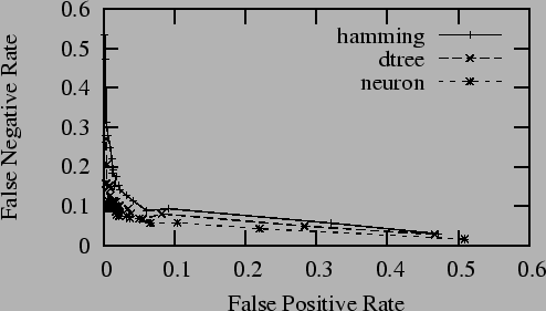
An important tradeoff in spam filtering is between false
positive (ham messages flagged as spam) and false negative
(misses, spam messages flagged as ham) rates. A
detector that always says ``ham'', after all, will never
experience a false positive. In communications theory,
this tradeoff is illustrated by a receiver operating
curve that shows the tradeoff between rates. Most spam
filters prefer to operate with a bias that minimizes the
total error. False positives, however, are generally much
more expensive than false negatives, so it may be
desirable to operate the filter outside of its optimal
range. Figure 3 shows receiver operating
curves for several spam filters on the synthetic corpus
discussed below. The spam filters were biased by varying
the percentage of spam from 5% to 95%: for these
filters, this caused the detection profile to shift. The
strong preference of the filters for operating with a
particular optimal bias is notable.
Figure 3:
Receiver Operating Curves
 |
The accuracy of the corpus is also a concern. It is to be
expected that a certain amount of misclassification of
messages and mis-recognition of features will be present
in the data. Section 7 discusses some of
the characteristics of the corpora used here. While these
corpora have received a great deal of attention from a
variety of sources, they nonetheless seem to have some
residual misclassification.
Different learners may cope with different types of
features and classifications. Ultimately, spam filtering
tends to concern itself with a binary classification: ham
vs. spam. More sophisticated document classifiers can
provide both more detailed classification outputs (e.g.
``Nigerian spam'', ``message from Mom'') and more precise
estimates of their classification confidence.
Some machine learners (notably neural nets) can handle
continuous feature values. Many learners are restricted to
discrete feature domains, and one of the algorithms
discussed here is tailored to binary features. The
learning algorithms described in this paper have been set up
to use binary features, for several reasons. The fact
that binary feature data can be handled by essentially any
inductive learner permits the comparison of a wide range
of approaches. The binary-feature version of a typical
learning algorithm is easier to explain: the mathematical
notation is complicated enough without worrying about
many-valued features. Perhaps most importantly, the
common types of binary feature detectors are more difficult
for a spammer to manipulate. For example, if the number of
occurences of a particular feature in a given message is
considered, a spammer can load a message up with repeated
instances of a ``good'' feature and overwhelm the
spam-related features of the message.
There are a huge range of approaches to machine learning
discussed in the literature. Several criteria have been used
to select algorithms for presentation:
- Simplicity: First and foremost, the
algorithm must be comprehensible and easily
implementable by UNIX developers of freely available software.
Algorithms comprehensible only to machine learning
experts have been eschewed: they often offer only a
marginal increase in performance in any case.
- Currency: Most of the algorithm families currently
being used by freely-available spam detectors are represented
in this sample. A glaring omission is genetic
algorithms. The range of algorithms and implementations
in this category is enormous, making it difficult to
select a canonical candidate. In addition, the
performance of genetic algorithms in spam filtering does
not currently appear to be exceptional.
- Pedagogy: The algorithms presented here are
those that are commonly used in introductory artificial
intelligence and machine learning
texts [15,5] to
introduce various classes of learners. While much more
sophisticated variants of each technique presented are
possible, grossly speaking the performance gains over
these simple techniques are modest, and the extra
implementation difficulties substantial.
It is worth emphasizing this last point again. More
sophisticated variants of each of the algorithms presented
here have already been applied to spam filtering.
Simple algorithms
tend to perform reasonably well, so focusing on
them is practical. More importantly, the
study of simple algorithms is intended to be inspirational,
leading to further investigation by spam filtering
practitioners in the freely available software community.
As mentioned earlier, this paper considers binary features
for binary classification. A feature detector is applied
to an e-mail message to produce a set
 of binary features of the message. The binary
classification of binary features of the message. The binary
classification  of the message may be given or may be
the quantity to be determined: this classification is
either of the message may be given or may be
the quantity to be determined: this classification is
either  indicating spam, or indicating spam, or  indicating ham. Both
the classified feature detector output indicating ham. Both
the classified feature detector output
 and the original e-mail message are informally referred to
as an instance. In the absence of other context the
feature detector output will be implied. Negation will be
represented with an overline, thus
and the original e-mail message are informally referred to
as an instance. In the absence of other context the
feature detector output will be implied. Negation will be
represented with an overline, thus
 is true when
feature is true when
feature  is absent. is absent.
The instances considered here are drawn from up to three
disjoint sets: a set  of training instances, a set of training instances, a set  of validation instances, and a set
  of classification
instances. When more than one instance is involved,
additional subscripts for features and classifications will
represent the instance; for example of classification
instances. When more than one instance is involved,
additional subscripts for features and classifications will
represent the instance; for example
 . The set of positive and negative
instances drawn from a set . The set of positive and negative
instances drawn from a set  will be
represented by will be
represented by  and and  respectively. The set of
instances with feature respectively. The set of
instances with feature  true and false will be
represented by true and false will be
represented by  and and
 respectively. respectively.
2 Techniques
In this section, several supervised learning techniques
are considered. An extremely simple baseline algorithm is
presented, intended partly to illustrate concepts and to
provide a standard of comparison. A discussion of
commonly-used and important algorithms ensues, concluding
with a decision-tree method. Finally, an advanced
approach using multilayer neural networks is discussed.
The authors have made UNIX utility implementations of each
of the algorithms described in this section freely
available: see Availability at the end of this
document. The corpus data used is also freely available
from the authors. (The exception is personal e-mail
messages, for which only feature data is available.)
Thus, the performance measurements reported in
Sec. 8 below should be readily
replicable by other investigators.
Perhaps the simplest conceptual method of learning is
as follows. When presented with the feature set  of a target instance to be classified, find a
subset
of a target instance to be classified, find a
subset  of the instances in the training set with
the same feature values . Then classify
if of the instances in the training set with
the same feature values . Then classify
if  , and , and
 otherwise. (Actually, ties should be
randomized appropriately.) otherwise. (Actually, ties should be
randomized appropriately.)
This brute-force method is simple to implement, but it has
drawbacks. Foremost of these is that given a reasonably
small training set and reasonably large number of
features, it may be unlikely to find any training
instances whose features match those of the target
instance. In this situation, the error rate may be very
high.
Minimum Hamming Distance Voting (MHDV) is an adaptation of
this ``brute force'' method designed to achieve
higher accuracy for a given training set size.
The Hamming distance
 between two binary vectors
and between two binary vectors
and  is defined to be
the number of bit positions in which and
differ. Thus, is defined to be
the number of bit positions in which and
differ. Thus,
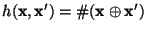 , where , where  is the exclusive-or operator and is the exclusive-or operator and
 is the population count or Hamming weight: the number
of 1 bits in the vector. is the population count or Hamming weight: the number
of 1 bits in the vector.
MHDV
generalizes brute force learning via the simple mechanism
of using nearby instances rather than identical ones.
Consider a target instance and a training set .
Let
be the subset of with minimal Hamming distance
from . A
target message is classified as spam if
and ham otherwise. Ties are broken randomly.
Formally, MHDV is an instance-based learning method,
specifically a  -nearest-neighbor algorithm with -nearest-neighbor algorithm with
 . Figure 4 illustrates the MHDV
classification process: the target instance (the empty
dot with feature vector . Figure 4 illustrates the MHDV
classification process: the target instance (the empty
dot with feature vector  )
is classified
positive in accordance with the majority of its distance-2
neighbors. )
is classified
positive in accordance with the majority of its distance-2
neighbors.
Figure 4:
MHDV Classification
 |
To the best of the authors' knowledge, instance based
learning has not previously been proposed as a spam
filtering methodology. There are serious advantages to
this approach, but also serious drawbacks. The accuracy
of MHDV improves dramatically as a function of the size of
, and therefore as a function of the size of . But
in a naïve implementation a single classification
requires comparing the target to each instance in
, and thus time  where where  is the number of
features. (More sophisticated implementations can use
similarity hashing techniques to improve this performance
somewhat.) The storage of the large set of instances is
also a burden, although storage is increasingly
inexpensive. is the number of
features. (More sophisticated implementations can use
similarity hashing techniques to improve this performance
somewhat.) The storage of the large set of instances is
also a burden, although storage is increasingly
inexpensive.
Note that reinforcement learning is easy with MHDV: simply
put misclassified instances into the training set with the
correct classification. MHDV should be easily extensible
to discrete or continuous features that obey a distance metric.
An interesting class of supervised learning algorithms
focuses on probabilistic interpretation of training data.
One of the simplest of these is the so-called naïve Bayesian approach. Bayes' Rule famously notes that
where
 is the probability that an instance is
spam given that it has the given feature set, is the probability that an instance is
spam given that it has the given feature set,
 is the probability that it has the given feature set
given that it is spam (an important distinction),
is the probability that it has the given feature set
given that it is spam (an important distinction),
 is the overall probability that a message is spam, and
 is the probability of receiving a
message containing the given features.
Crucially,
the quantities on the right-hand side of the equation can
all be measured, under the (wrong, but surprisingly
harmless in practice) assumption that the features is the probability of receiving a
message containing the given features.
Crucially,
the quantities on the right-hand side of the equation can
all be measured, under the (wrong, but surprisingly
harmless in practice) assumption that the features
 are independent, having no
particular statistical relationship.
A Naïve Bayes classifier thus classifies a message as
spam when are independent, having no
particular statistical relationship.
A Naïve Bayes classifier thus classifies a message as
spam when
Note that the denominator is constant across the
inequality and can be dropped.
Some algebraic
and probabilistic manipulation
yields a decision rule that classifies a message
as spam
if and only if
To oversimplify, Naïve Bayes
classifies an instance as spam if it shares more
significantly in the features of spam than in the features
of non-spam. The rule also takes into account the
a priori probability that the message is spam, i.e.
the overall spamminess of the training set. A statistical
adjustment (see [15]) is used for features that appear rarely or
not at all with a given sign in the corpus. It is also
common to take logarithms to turn the product computation
into a sum computation: this greatly improves numerical
robustness at a slight expense in performance.
The Naïve Bayes classification
rule can be seen as a relative of the MHDV rule
that uses the feature set in a different, more principled
fashion. Another major difference is that the set sizes used in
the decision rule can be computed during the learning
phase, and the training data then discarded. This makes
classification more efficient than with MHDV.
Naïve Bayes learning is relatively simple to implement,
and accommodates discrete features reasonably well. It is
not quite as accurate or robust as some other methods, but
is highly efficient to train. Reinforcement learning is
also easy: the relevant set sizes are simply continuously
updated with newly-classified instances.
3 Graham
As mentioned earlier, much of the interest in Bayesian
methods in the freely available software community was
inspired by Graham's article A Plan For
Spam [6]. The machine learning approach
used by Graham was an informal probabilistic one:
Robinson [18] later elucidated the
relationship between Graham's technique and Naïve Bayesian methods.
In essence, Graham's method is similar to Naïve Bayesian: the a priori probabilities of a message's
words are combined to yield a likelihood that the
message is or is not spam. Specifically, Graham
classifies a message as spam if
is greater than  . The features used in the
calculation are those words whose contribution to the
product differs most from . The features used in the
calculation are those words whose contribution to the
product differs most from  : roughly speaking, these are
the high-gain words (Sec. 4.2.5). Various
empirical adjustments are made to the above formula in the
implementation:
Graham asserts that they do not change the
classification except in unusual cases. : roughly speaking, these are
the high-gain words (Sec. 4.2.5). Various
empirical adjustments are made to the above formula in the
implementation:
Graham asserts that they do not change the
classification except in unusual cases.
Robinson has designed an adapted Bayesian method that is
claimed to be a strict improvement on Graham's approach:
true Naïve Bayesian is supposed to be better yet,
although it often seems to offer only a small improvement
in experiments reported here. Graham's success in spam
filtering shows that even an extremely simple and
less-principled approach to spam feature detection and
machine learning can get good results in practice.
4 Perceptron
Figure 5:
Artificial Neuron
 |
Neural nets are commonly used in supervised learning.
The simplest form of neural net is the
single-element perceptron: a message is classified
as spam if and only if
where the  are real-valued weights.
Note that the output is made binary by thresholding: in
addition to being convenient for a binary classifier, this
non-linearity is important in building larger neural networks.
Figure 5 shows the perceptron structure
schematically. are real-valued weights.
Note that the output is made binary by thresholding: in
addition to being convenient for a binary classifier, this
non-linearity is important in building larger neural networks.
Figure 5 shows the perceptron structure
schematically.
The weights are assigned during the training phase by
gradient descent. Repeated passes are made over all
training instances: small adjustments are made to the
weights on misclassified training instances until the
number of misclassified validation instances is minimized.
This somewhat awkward procedure minimizes the probability
of overtraining the perceptron.
Multilayer neural nets use the output of single
perceptrons or similar structures as inputs to subsequent
perceptrons. This allows the system to learn more complex
features, at the expense of more complex training and
difficult control.
Perceptrons and other artificial neurons accommodate
binary and discrete features essentially by treating them
as continuous. Reinforcement learning in
these systems is by adjusting the training weights to
correctly reclassify misclassified instances.
5 ID3
Decision tree learning is a bit more complicated than the
above methods. The ID3 decision
tree algorithm [17] is a simple, classic decision
tree learner. The information-theoretic entropy  of a set of messages represents the difficulty of
determining whether a message in is spam or non-spam:
of a set of messages represents the difficulty of
determining whether a message in is spam or non-spam:
where
If is partitioned based on the value of some
particular feature , so that
 , the information-theoretic gain , the information-theoretic gain
represents the information gained by considering the subsets
and
separately.
In ID3 the feature
yielding the highest gain on the training
set is selected for splitting. These subsets
are further split until subsets are produced containing
instances of only one or largely a single classification. The resulting tree
is used in
the classification stage: target instances are given the
classification matching that of the training instances in
their leaf subset. Overtraining is controlled by stopping
the split when the largest gain is small, or when the
statistical significance of a split as given by a  test is
too low. Figure 6 shows a binary decision tree:
an instance is classified by walking from the root of the
tree to the leaf, choosing a direction at each node based
on the properties of the given feature. Since the given
instance has feature 3 positive and feature 2 negative, it
will be classified as ham. test is
too low. Figure 6 shows a binary decision tree:
an instance is classified by walking from the root of the
tree to the leaf, choosing a direction at each node based
on the properties of the given feature. Since the given
instance has feature 3 positive and feature 2 negative, it
will be classified as ham.
Figure 6:
Decision Tree
 |
Decision trees can easily accomodate multi-valued discrete
features by way of  -ary trees. Continuous features are
usually handled by quantization. Reinforcement learning
usually involves simply putting the newly-classified
instance at the appropriate leaf: occasionally tree
operations may have to be performed to preserve the
property of splitting on the highest-gain features first. -ary trees. Continuous features are
usually handled by quantization. Reinforcement learning
usually involves simply putting the newly-classified
instance at the appropriate leaf: occasionally tree
operations may have to be performed to preserve the
property of splitting on the highest-gain features first.
In addition to the relatively unsophisticated techniques
described above, more advanced machine learning techniques
can also be used to filter spam. In general, these
techniques trade off more complex and difficult designs
and implementations for potentially higher quality
results. This study explores one such
approach as an example: constructing a multilayer neural
network. This methodology generalizes the simple
perceptron of Section 4.2.4, and provides a
good illustration of the tradeoffs of an advanced machine
learning approach for spam detection.
When constructing a multilayer neural network, one is faced with the
choice between implementing from scratch, or attempting to
use an existing package that is freely
available. Implementing a neural network from scratch is
appropriate when performing neural network research:
however, it requires substantial effort to develop and debug
it, and more effort still to validate it. Subtle numerical
bugs can easily contaminate data in ways which are difficult
to detect.
Given a focus on spam filtering research rather than
neural network research, a free software platform is a
natural choice. Using free neural network software
leverages years of development and debugging
effort. Because free software is in widespread use by
researchers around the world, it undergoes intense
scrutiny for correctness, and bugs can be fixed quickly
when they are found. The availability of the software
makes it easier for other researchers to reproduce and
extend results. One caveat, however, is that a firm grasp
of the principles behind neural networks is still
necessary. Neural networks are sometimes finicky learners,
and can produce poor results when improperly constructed
and used.
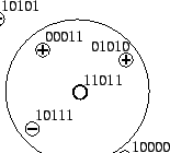
A neural network consists of multiple, interconnected computational
units. Each unit can have multiple inputs, but only a single
output. The unit's basic function is to add up the values of its
inputs, and transform the result with a nonlinear function to produce
its output. The individual units are not very powerful by themselves,
but when linked together in a network they can carry out complex
computations.
Although each unit can only produce a single output value, this value
can be used as input to many other units. Connections between the
output of one unit and the input of another are called links. Each
link has an associated weight. The output of the first unit is
multiplied by this weight to become the input of the second unit. In a
network with hundreds of units there can be thousands of links, and
therefore thousands of weights. It is these weights which change as
the network is trained.
Figure 7:
Neural Net
 |
The network configuration used for spam filtering was a
basic feedforward topology. In this configuration, the
network can be viewed as a series of layers of units
with the outputs of one layer fully
connected to the inputs of the next layer.
This topology is
called feedforward because there are no loops (links only go
forward, never backward) and no jumps (links never skip over
intervening layers). The input cascades from layer to layer,
undergoing a transformation at each step, until it becomes
the output. The first layer of the network is the input
layer. This layer collects the input and passes it through
weighted links to the first interior hidden layer.
Each hidden layer computes the weighted sum of its inputs,
and then transforms the resulting values with a nonlinear
transfer function to produce its output. The last
hidden layer sends its output to the output layer,
which in some configurations may apply a final nonlinear
transformation. In our network, the output layer did not use
a nonlinear transfer function.
Figure 7 shows one such network, with three
input neurons, two hidden neurons, and one output neuron.
Figure 8:
Sigmoid Response Function
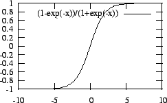 |
The nonlinearity of the hidden units is what gives a neural
network its power to learn complex functions. Without some
form of nonlinearity, the transformations performed by the
layers of the network amount to nothing more than a series
of matrix multiplications; a multi-layer network would be
equivalent to our simple perceptron. Thus it is necessary
to introduce nonlinearity if the network is to be able to
learn complex mappings. For our networks we selected a
transfer function called the sigmoid,
an S-shaped curve whose graph is shown in
Figure 8.
This function
is commonly used in neural network research, and should be
available in any free or commercially available neural
network package.
In the feedforward networks employed in this project, the
input layer consists of a number of units equal to the
feature vector size of the input: each input unit
corresponds to a single feature. Because we are treating
spam detection as a binary classification problem, only one
output unit is used. The output of this unit should be 0 for
nonspam inputs, and 1 for spam inputs. Note that, as with
the perceptron, it is possible to allow the neural network
output to vary continuously, indicating the likelihood that
a message is spam: this provides one way to trade off false
negatives for false positives, while flagging marginal
messages for further consideration.
One of the trickier tasks in constructing a multilayer
neural net is choosing the number of hidden layers and the
number of units in each layer. The spam filter design
uses a single hidden layer with many fewer units than the
input layer. It is desirable to have as few hidden units as
possible to avoid a form of overfitting in which the extra
neurons end up modeling unimportant training set details.
However, with too few hidden units, the network will not be
able to accurately model the underlying function.
The weights in large networks correspond to a large number
of degrees of freedom. Estimating how many degrees of
freedom are truly necessary involves estimating the degree
of correlation between inputs. It is easier to estimate the
number of degrees of freedom if the inputs are as
uncorrelated as possible. A word clustering feature
detector (Sec. 5.3) helps to achieve this
by dividing words into clusters which are maximally
independent.
Like the perceptron, a neural
net is trained through a process of adjusting the link
weights between layers so as to bring the actual output
vectors closer to the desired ones. The network essentially
learns "by example." The most famous training algorithm for
feedforward networks is backpropagation. In backpropagation,
values first flow forward through the network to produce
outputs. These outputs are compared with the desired ones,
and errors are then propagated backward through the network,
adjusting the weights so as to reduce the error.
A closely related training technique, Rprop,
has many of the same features as backpropagation: it was
selected for filtering because of its robustness and quick
convergence.
Several issues arise when selecting a
network design. It is clear that the input layer must have
as many units as the number of features in the feature
vectors, but these value can be presented to the network in
different ways. Simplest is to treat each feature as a binary
input, which is 0 when the feature is not present, and 1 if
it is, regardless of how many times that feature might occur
in a single message. This makes the neural net compatible
with the other machine learners discussed here, and
simplifies feature processing.
(Another option would be to standardize the input values
according to some statistical model. Originally,
the input values were standardized under the
assumption that they are normally distributed. The purpose
of this was primarily to accelerate the learning of the
network. Because the feature counts have a wide
spread--many are 0, some can be in the hundreds--it takes
a long time for the network to adjust its weights to account
for this spread. Standardizing the inputs brings the values
closer together, which speeds convergence.)
SNNS is a neural network simulation package developed at the
University of Stuttgart in Germany. The source code is open,
and the software is freely available for research and
academic use. The homepage of the SNNS project can be found
at https://www-ra.informatik.uni-tuebingen.de/SNNS/.
SNNS was selected for many reasons. Most important is its
great flexibility. SNNS supports a wide range of network
topologies, not just feedforward networks. It provides an
array of training algorithms which can be applied to almost
any kind of network design. Parameters like the number of
layers, layer dimensions, links, and transfer functions are
all fully configurable. This allows experimentation with a variety of
designs with no time wasted recoding the network.
SNNS has a very attractive GUI which runs under X. Although
there is no visual design tool, it is straightforward to
configure a basic feedforward network. The GUI can display
the network in action and can produce graphs of output error
over time. These features make it simple to visually
determine when the network is performing well.
The package can also be operated in a batch mode. The batch
interpreter has a complete scripting language to automate
training sessions. Training and validation can be scheduled
arbitrarily, and error results can be written to disk at any
time during the process. This makes it simple to begin
training runs on large datasets overnight.
Finally, SNNS has the ability to translate a trained network
into a C program. Although the network cannot be trained
further once converted to C, it is very compact and easily
callable from other C code. This makes it possible to build
high-performance message classifiers once the network is
trained.
The use of an open source neural network ``construction
kit'' thus permits simple implementation of a quite
sophisticated machine learner for spam. A similar approach
could be employed for other machine learners discussed
earlier, as open source construction kits are available for
a wide variety of machine learning techniques.
The problem of feature detection is largely orthogonal to
the problem of learning on the identified feature set.
(This observation does not seem to be commonly made in the
open source community, and deserves wider attention.)
This work has experimented with several different types of
feature detector. More sophisticated methods have been
applied to feature detection. For example, Lewis' Data
Enrichment Method [13] is unbelievably
powerful, but has other drawbacks that prevent its use in
the real world.
The feature set computed by SpamAssassin was the initial
basis of this study. The advantages of this approach are
manifold: SpamAssassin provides several hundred
hand-crafted binary features, the
features seem to be reasonably sensitive, and using
SpamAssassin features permits easy comparison with the
classification performed by SpamAssassin
itself.
The features recognized by SpamAssassin provide a fine
feature source for the learning algorithms described
above. Maintenance of this feature detector, however, is
a tremendous amount of work. In addition, the detector is
quite slow, as slow as a few messages per second if the
network-based lookup features are enabled.
Rather than hand-crafting a feature detector, it would be
useful to automatically extract features directly from the
corpus. When trying to classify email the most natural
features are the words of the message. A standard
approach is to use individual words directly as
features. Each feature vector element indicates whether a
particular word is present in a message. However, the
English language contains thousands of words, while every
email message contains only a small subset of those
words. This makes it difficult to decide which words are
good representatives of spam mail and nonspam mail, given
a limited amount of features.
To this end, a feature detector has been constructed that
selects e-mail body words with the highest
information-theoretic gain (Sec. 4.2.5) as likely
high-utility candidates for learning algorithms. This
detector appears to work quite well, with learning
accuracies approaching those achieved with the
SpamAssassin detector. The detector operates by breaking
the e-mail body into words using simplistic rules, and
then measuring the gain of each word using a dictionary.
Those words with gain above a set threshold are retained.
3 Word Clustering
A preliminary attempt was made to
assess the performance of word-based features, using
the 134 words with the highest
information gain as features. The resulting feature vectors
were quite sparse: most messages had few high-gain words. The training cost
of supervised learning algorithms generally grows in proportion to the
number of inputs. For example, the number of weights
in a feedforward neural network grows in this
fashion. Because training time is proportional to
the number of weights, considering a large number of inputs
can make training intractably slow. What is needed, then
is a way to automatically extract a small number of
features that nonetheless give a strong signal on every message.
One solution to this problem is to cluster words of similar
meaning together into a single feature. This allows more
unique words (thousands instead of hundreds) to be considered
when scanning a message for features, while simultaneously
keeping the feature count low enough to make training
managable. This gives much better coverage of the set of
words occurring in email messages.
An information-theoretic clustering algorithm described in
a recent paper by Dhillon and
Modha [4] seems to be a good candidate.
This algorithm was selected from among many other
clustering algorithms proposed for machine learning
primarily because its execution time is linear in the
number of words and clusters. Other clustering techniques
tend to be quadratic or worse in the number of words and
clusters. In addition, the Dhillon algorithm is unlike
some other clustering algorithms in that it considers the
spam/non-spam classification of the messages while clustering. The
mechanics of the Dhillon algorithm are briefly described
here; the original paper by Dhillon gives a deeper look at
the information-theoretic concepts underlying it.
The initial assignment of words to clusters is done by
allocating two sets of empty clusters of equal size. Words
which occur more often in nonspam messages are randomly
assigned to one of the ``ham clusters''. Similarly, spam
words are assigned to a spam cluster. This concept of
nonspam clusters vs. spam clusters is only meaningful during
initialization, since the clustering algorithm will move the
words between clusters to minimize the clustering metric. In
the final clustering, some clusters may contain both ham
and spam words.
After the initialization step the algorithm becomes
iterative. On each pass through the loop words are moved
between clusters to decrease the value of a divergence
metric. This metric quantifies the average dissimilarity
of the words in each cluster. Minimizing this value
thus maximizes the intra-cluster similarities. Iteration
then continues until the divergence metric does not change
more than a fractional amount from the previous iteration.
The implementation of the clustering algorithm is done in
three major blocks: collection of data, clustering of
data, and output of clusters. Each message body is
initially scanned and tokenized into words. The
clustering function takes as input the desired number of
clusters. The clusters are initialized as described
above. To reduce the number of candidate words to a
manageable size, the implementation only considers words
which occur more than a minimum number of times over all
the messages.
The iterative algorithm then executes. After a number of
iterations
the clustering converges. The number of
clusters output by the algorithm may be less than
requested, because some clusters become empty during the
iteration of the main loop. Only non-empty clusters are
output at this phase.
The final step is generating the feature vectors. Using
the cluster file generated by the clustering algorithm,
each message body in the corpus is again scanned, matching
each scanned word to its cluster. This is done by loading
the cluster file into a hash table which maps each word to
its cluster number, which is a nearly constant-time
operation. Since each word in the message must be
examined once, the time it takes to scan a message is thus
roughly linear in the number of words in the message.
It is sensible to consider combinations of feature
detectors. The comparison is complicated. As noted
previously, larger feature sets slow recognition and
learning: it may be better to use more features of a given
type than to combine features of several types.
For the feature detectors examined here, combinations are
less problematic. The SpamAssassin detector operates on
header information (and by all accounts does well at
this): the other detectors operate only on body
information. The clustering detector is believed to
perform strictly better than the gain-based detector,
since it is essentially a superset of it. Thus, there are
five combinations that are leading candidates for
examination: the three detectors alone; SpamAssassin plus
gain-based; and SpamAssassin plus clustering.
Work on text classification in general, and spam detection
in particular, dates back many years in the machine
learning community. For example, Androutsopoulos has
worked with a number of researchers on machine learning
spam filters [1,19]. A good
overview of machine learning for e-mail classification
is in Itskevitch's M.S. Thesis [9].
These approaches first caught the wide attention of the
open source community with Graham's web article
(Sec. 4.2.3). This article and Robinson's
commentary on it inspired a number of implementations of
semi-Bayesian word-based filters, many of which can be
found at sourceforge.net.
At the same time, non-learning-based approaches to spam
filtering have also been widely attempted. The
SpamAssassin tool is a freely-available Perl-based spam
filter that combines hand-crafted features using a
perceptron. Initially, the perceptron weights were
hand-tuned: more recently, a genetic algorithm was used to
train the weights on a synthetically composited corpus.
Oddly, the SpamAssassin authors have apparently not
used a traditional gradient-descent approach to tune their
perceptron: it was this omission that inspired the authors
of this paper to begin the research reported here.
SpamAssassin combines its primary feature data with other
sources of information, such as spam databases and
word data, to produce a final classification.
7 Corpora
The problem of selecting a corpus for evaluation of
learning algorithms for spam detection is a difficult one.
One challenge is that private e-mail is rarely available
for public study: thus, other sources of ham must be
found if the corpus is to be made publically available.
For evaluation purposes, four corpora were assembled.
The first corpus consists of the first author's e-mail
over a recent two-year period, a total of 15,498 messages.
These messages were randomly sampled to select exactly
15,000 messages for ease of use. This corpus has the
advantage of verisimilitude: most studies have used only
corpora consisting of synthetic combinations of messages
from public mailing lists and spam databases. The corpus
is about 50% spam: a percentage higher than indicated in
older publications on the subject [3], but
consistent with current anecdotal evidence. For privacy
reasons, the corpus itself is not publically available:
however, the instance data derived from the corpus by
feature recognition is.
The second corpus is a total of 15,000 messages drawn
equally from two sources: 50% of the messages are
ham from the X Window
System developer's Xpert mailing list; 50% are spam from
the Annexia spam archive [2]. The a
priori accuracy rate of this corpus is much lower; there
are frequent classification errors in both data sets.
This corpus is publically available.
The third corpus is the Lingspam corpus, a synthetic
corpus of 2405 messages. 80% of these messages are
ham from a linguistics mailing list: the rest is spam.
The corpus has been made publically available by Ion
Androutsopoulos, and used in publications by several
authors: it thus provides a basis for comparison with
published work.
The fourth corpus is used to tune SpamAssassin, and
consists
of 8686 messages, 80% ham and the remainder spam, from
a variety of sources. It is deemed useful for comparison
with a fielded freely-available spam filter, as well as
being a robust corpus useful in its own right.
8 Evaluation
Each of the algorithms reported in
Sec. 4.2 has been implemented in C and
Perl by
the authors. These implementations are freely available
as noted at the end of this document.
Accuracy and speed of the implementations
have been measured on a 1.8AGHz AMD box with 512MB of main memory,
running Debian ``Woody'' with kernel 2.4.19.
The preliminary nature of the measurements reported here
should be emphasized. There are an enormous number of
interesting experiments that can be run given the sample
setup, and there is an enormous amount of work that can be
done to improve the design and implementation of these
spam filters. Nonetheless, the measurements in this
section serve both to provide a gross comparison between
various learners and detectors, and to illustrate some of
the issues that arise in practical machine learning.
Figures 1, 2
and 3 show some of the measurements made.
Those measurements are good illustrations of the power of
experimental data in elucidating machine learning issues.
Table 1 shows the classification accuracy
of the algorithms on the sample corpora.
The columns
labeled and T are false positive and
total error percentages respectively. (The false positives
are shown as percentage of total messages, rather than
percentage of ham messages; they thus reflect the mix of
messages in the given corpus.)
The columns labeled SA, BD, and CL denote the
use of the SpamAssassin, Body Dictionary, and CLustering
feature detector: the SA+BD and SA+CL columns denote the use
of combined feature sets.
All programs were run using default parameter settings.
Statistics
reported are worst of 10 runs, in accordance with PAC
theory [21]. Two-thirds of the corpus have been
used for training (and validation when required), while
the final third has been used for classification: a new random
split has been used for each run, with all programs being run
over the same 10 splits.
The gain threshold of the body word detector was selected
to give a maximum of a few hundred features across all
corpora. This seemed to give sufficient accuracy for
evaluation purposes, but more experimentation in this area
would be prudent.
Table 1 is unfortunately difficult to read.
Nonetheless, it contains a great deal of useful data, from
which several conclusions can be drawn.
While the differences between classifiers and between
feature detectors are quite significant, it can fairly be
said that overall the accuracy of the filtering systems
is similar. The exceptions reveal a number of interesting
phenomena.
The more complex classifiers seem to be consistently
better than the simpler ones. In particular, the neural
net is the most consistently strong classifier: the decision
tree learner also produces good results. As expected, the
combined feature detectors tend to be stronger overall
than their components: the SA detector appears to work
well with most classifiers and corpora.
Specific classifiers seem to have trouble with specific
corpora or detectors. Note
particularly the 100% false negative rate of the graham
classifier on the personal and synthetic corpora with the CL
detector. It is believed that this anomaly is not a
program defect, but results from a peculiarity of the CL
feature set: for these large inputs, the detector tends to
group all of the spam words into just one cluster, while
the ham words have a large number of clusters.
Graham's heuristic does not cope well with this case: the
large number of ham features swamps the signal from the
much more significant spam features.
The graham classifier appears to be less strong than
the nbayes classifier overall, but not dramatically
so: the choice of corpus and features appears to matter significantly.
The hamming detector appears to be a good, reliable
detector overall, and may actually be a reasonable choice
in situations where its slow classification rate can be
reduced or ignored.
Table 2:
Feature Detection Time
| |
s/Kmsg |
s/MB |
| SA |
1784 |
391 |
| BD |
15.2 |
1.9 |
| CL |
14.0 |
1.7 |
Table 2 shows feature detection time for
the synthetic corpus. The BD classifier gain
threshold is 0.05. Times shown are wall clock seconds per
1000 messages and seconds per megabyte (1,048,576 bytes).
Neither the BD nor the CL detector is significantly optimized
for performance--significant improvements could be
expected in practice. These times suggest why work on
alternate feature detectors and an overall move away from
SpamAssassin may be important in the future.
Table 3:
Training and Classification Time
| |
T |
C |
| hamming |
0.00 |
44.05 |
| nbayes |
0.65 |
0.06 |
| graham |
0.65 |
0.02 |
| neuron |
10.66 |
0.00 |
| dtree |
5.45 |
0.00 |
| net |
140.35 |
0.13 |
Table 3 shows
training and classification time for the synthetic corpus
and SA feature detector.
Training and
classification times are exclusive of feature detection
and other times. All times are CPU seconds per 1000 instances,
and are the average of 10 runs.
Times shown as 0.00 are less than 0.01 seconds per 1000
instances, in other words in excess of 100,000 instances
per second.
As expected, the neuron and dtree detectors require a
moderate training period. The net detector is
slow to train (although not unusably so). The hamming detector as implemented is probably too slow to
use for server filtering, although it would work fine for
filtering an individual's messages.
The initial integration target for the work described here
has been SpamAssassin, a
rule-based mail filter written in Perl by a team including
Justin Mason. SpamAssassin is an open source project distributed under
Perl's Artistic license: it was hoped that it would
be a good basis for
third-party extension. The mechanism by which
SpamAssassin classifies a message is via handcrafted
header and body text analysis rules, along with
blacklist/whitelist support (lists of addresses to
automatically deny or accept) and use of a spam tracking
database such as Vipul's Razor. After the test suite has been
run, the mail message can optionally be marked with a spam
header for easy processing by a user's mail reader. The
package is primarily made up of libraries of test and mail
handling code, forming an API that allows for easy
integration with mail applications on multiple platforms.
Various command line and
daemon scripts for interfacing with the API are also supplied.
The SpamAssassin API libraries consist of two main sections:
code to run each of the tests, and the engine that calls the
test code and combines (and scores) the results. The text
analysis portion of the testing code is comprised of regular
expressions that are matched against the headers and body of the mail
message. SpamAssassin allows for quite a bit of flexability
by coding many of the tests in user editable configuration
files--tests can thus be added or modified without change to
the Perl libraries themselves. Unfortunately, the format of
the configuration file only allows for the specification
of new tests involving single regular expressions.
The classification engine is responsible for handling mail input
and output, including mail message headers and body text.
It also supports routines to update test parameters. For example,
adding and removing mail addresses from accept and deny
lists, or reporting a mail message to collaborative spam
tracking databases online. After running the full suite of
classification tests, the testing engine scores the mail message based on
the results of each of the tests. If the message is
classified as spam the engine takes appropriate action, such
as rewriting the mail message to include easily recognizable
tags for the user in the subject line and message body, as
well as adding an extra header for the user's mail
user-agent to automatically refile spam messages.
Recently, the SpamAssassin team has added support for
classification of mail messages using a ``Bayesian-like form
of probability-analysis'', apparently based on a
Graham/Robinson (Sec. 4.2.3) or Naïve Bayes
detector. This extension seems to allow for online learning
and storage of new message characteristics, although the
documentation is incomplete at the time of this writing.
While the Bayesian extension appears to implement the same
algorithm as the Naïve Bayesian classifier described here,
it is embedded in the SpamAssassin code. This makes it hard
to inspect, and requires modifying the SpamAssassin code
itself to make changes.
One straightforward way to integrate the classifiers with
the SpamAssassin package is to convert them to Perl.
Currently the perceptron learner has been completely
converted and an offline classification mode has been
implemented. The SpamAssassin feature set is used as
training input to this learner. The other learners are
only partially integrated: the classification phase is
available to SpamAssassin.
A SpamAssassin-style manually-weighted
perceptron is used to integrate the
classifiers, including
SpamAssassin's built-in classifier.
New feature detectors can be integrated with the setup and
used by all of the learning classifiers.
Modifications to the SpamAssassin code have been kept as
minimal as possible. Code implementing a linear perceptron
has been added to the check() method of the Mail::SpamAssassin
module to allow as many classifiers to be run on a message
as desired: the result of each classifier is weighted in
a user-specified fashion. Parameters have been added to the new()
method of the module to select combinations of
classifiers and feature detectors, weights for the
classifier's output, and a perceptron threshold value
used
to make the final classification decision on the e-mail message.
Modifications have also been made to the
Mail::SpamAssassin::PerMsgStatus module. Parameters
have been
added to the new() method specifying the existing (and
allowable) feature detectors and classifiers. Each feature
detector is associated with the method implementing it as
well as the dictionary file required to create a feature
vector. Each classifier is associated with a file
containing state information required for classification (a
listing of current weights for the single neuron learner,
for example). Methods have been added to implement the feature
detectors, or retrieve the classification test results from
SpamAssassin's builtin feature detector, as well as to
encode the returned feature sets according to the specified
dictionary. A _psam_check() method has also been
added:
the method calls
the indicated classifier with the created feature vector and
returns the result.
As of this writing, the integrated system is close to being
ready to submit to the SpamAssassin team for review and
integration. Unfortunately, the runtime overhead associated
with the Perl implementation of SpamAssassin and the
learners and classifiers has proven to be a significant
problem. Thus, the direction to take from here is unclear.
Finding a simpler and more efficient open source framework
is currently under consideration as an alternative, as is
building yet another mail classification framework.
It has been said that good research raises more questions
than it answers. By that standard, the research reported
here has been successful indeed. Much more work is needed
on the corpora: it would be nice to establish a trustworthy
and representative test corpus of about 10,000 messages for
future work. Validation and tuning of both the feature
detectors and classifiers is badly needed to establish
confidence in their correctness and to understand ideal
operating parameters for them. Using ensembles of
detectors, detector biasing techniques, and other advanced
methods should be explored to improve accuracy. An
integrated mail-filtering system should be built, and
overall system accuracy and performance evaluated. An
anonymous referee of this paper suggested that the learners and
classifiers should be packaged in a library for use in
this and other projects: this is an excellent idea and will
be implemented.
Supervised machine learning is an effective technique for
spam filtering. The methods described in this paper provide
the basis for reasonably accurate, efficient classification
of messages as ham and spam. Freely-available software
implementors interested in spam filtering are encouraged to
take advantage of these techniques (and their more
sophisticated cousins) to help control the spam deluge.
Special thanks to: the Usenix Association
and the Portland State University Computer Science
Department
for enabling the student
authors of this paper to attend the conference;
Carl Worth for shepherding the paper;
Keith
Packard and Mike Haertel for help and advice (as usual)
with code and algorithms; and
Jeff Brandt for valuable ideas, criticism,
encouragement, and help with corpora.
The instance data and implementations used in this work are
freely available under an MIT-style license at
https://oss.cs.pdx.edu/psam.
- 1
-
Ion Androutsopoulos, John Koutsias, Konstantinos V. Chandrinos, George
Paliouras, and Constantine D. Spyropoulos.
An evaluation of naive Bayesian anti-spam filtering.
In G. Potamias, V. Moustakis, and M. van Someren, editors, Proceedings of the Workshop on Machine Learning in the New Information Age:
11th European Conference on Machine Learning, pages 9-17, Barcelona, Spain,
June 2000.
- 2
-
Annexia Spam Archive.
URL https://www.annexia.org/spam/index.msp accessed 25 November
2002, 22:00 UTC.
- 3
-
Lorrie Faith Cranor and Brian A. LaMacchia.
Spam!
Communications of the ACM, 41(8):74-83, August 98.
- 4
-
Inderjit Dhillon, Subramanyam Mallela, and Rahul Kumar.
Enhanced word clustering for hierarchical text classification.
Technical Report TR-02-17, Department of Computer Sciences,
University of Texas at Austin, Austin, Texas, March 2002.
URL https://citeseer.nj.nec.com/507920.html accessed 8 Apr 2003,
00:41:35 UTC.
- 5
-
Matthew L. Ginsberg.
Essentials of Artificial Intelligence.
Morgan Kaufmann, 1993.
- 6
-
Paul Graham.
A plan for spam.
URL https://www.paulgraham.com/spam.html accessed 18 November
2002, 22:00 UTC.
- 7
-
Paul Graham.
Better Bayesian filtering.
In Houbart [8].
URL https://spamconference.org/proceedings2003.html accessed 23
March 2003, 21:18 UTC.
- 8
-
Gilberte Houbart, editor.
Proc. 2003 MIT Spam Conference, Cambridge, MA, January 2003.
URL https://spamconference.org/proceedings2003.html accessed 23
March 2003, 21:18 UTC.
- 9
-
Julia Itskevitch.
Automatic hierarchical e-mail classification using association rules.
Master's thesis, Simon Fraser University, July 2001.
- 10
-
Paul Judge.
Spam research: Establishing a foundation and moving forward.
In Houbart [8].
URL https://spamconference.org/proceedings2003.html accessed 23
March 2003, 21:18 UTC.
- 11
-
Seth Kaplan.
How antispam software works.
Wired Magazine, 11(4):43, April 2003.
- 12
-
David D. Lewis.
(Spam vs. forty years of machine learning for text
classification.
In Houbart [8].
URL https://spamconference.org/proceedings2003.html accessed 23
March 2003, 21:18 UTC.
- 13
-
Henry R. Lewis.
The data enrichment method.
Operations Research, vol. 5, 1957.
Reprinted in J. Irreproducible Results 15(1), 1966, and in
subsequent collections from same.
- 14
-
Stanton McCandlish.
Archeology of spam.
URL
https://www.eff.org/Spam_cybersquatting_abuse/Spam/archeology_of_spam.article accessed 8 April 2003, 20:45 UTC.
- 15
-
Tom M. Mitchell.
Machine Learning.
McGraw-Hill, 1997.
- 16
-
Marco Paganini.
ASK: Active Spam Killer.
In Proc. 2003 Usenix Annual Technical Conference, San Antonio,
TX, June 2003.
To appear.
- 17
-
J. Ross Quinlan.
Induction of decision trees.
Machine Learning, 1(81):106, 1986.
- 18
-
Gary Robinson.
Spam detection.
URL
https://radio.weblogs.com/0101454/stories/2002/09/16/spamDetection.html accessed 18 November 2002, 22:00 UTC.
- 19
-
G. Sakkis, I. Androutsopoulos, G. Paliouras, V. Karkaletsis, C. D. Spyropoulos,
and P. Stamatopoulos.
Stacking classifiers for anti-spam filtering of e-mail.
In L. Lee and D. Harman, editors, Empirical Methods in Natural
Language Processing (EMNLP 2001), pages 44-50, Pittsburgh, PA, 2001.
- 20
-
SpamAssassin.
URL https://www.spamassassin.org accessed 18 November 2002,
22:00 UTC.
- 21
-
Leslie G. Valiant.
A theory of the learnable.
Communications of the ACM, 27(11):1134-1142, November 1984.
Bart Massey
2003-04-08
This paper was originally published in the
Proceedings of the
USENIX Annual Technical Conference (FREENIX Track),
June 9 – 14, 2003,
San Antonio, TX, USA
Last changed: 3 Jun 2003 aw
|
|
|