|
Security '05 Paper
[Security '05 Technical Program]
Mapping Internet Sensors With Probe Response Attacks
John Bethencourt
Jason Franklin
Mary Vernon
Computer Sciences Department
University of Wisconsin, Madison
{bethenco, jfrankli, vernon}@cs.wisc.edu
Abstract
Internet sensor networks, including honeypots and log analysis centers
such as the SANS Internet Storm Center, are used as a tool to detect
malicious Internet traffic. For maximum effectiveness, such networks
publish public reports without disclosing sensor locations, so that
the Internet community can take steps to counteract the malicious
traffic. Maintaining sensor anonymity is critical because if the set
of sensors is known, a malicious attacker could avoid the sensors
entirely or could overwhelm the sensors with errant data.
Motivated by the growing use of Internet sensors as a tool to monitor
Internet traffic, we show that networks that publicly report
statistics are vulnerable to intelligent probing to determine the
location of sensors. In particular, we develop a new "probe
response" attack technique with a number of optimizations for
locating the sensors in currently deployed Internet sensor networks
and illustrate the technique for a specific case study that shows how
the attack would locate the sensors of the SANS Internet Storm Center
using the published data from those sensors. Simulation results show
that the attack can determine the identity of the sensors in this and
other sensor networks in less than a week, even under a limited
adversarial model. We detail critical vulnerabilities in several
current anonymization schemes and demonstrate that we can quickly and
efficiently discover the sensors even in the presence of sophisticated
anonymity preserving methods such as prefix-preserving permutations or
Bloom filters. Finally, we consider the characteristics of an Internet
sensor which make it vulnerable to probe response attacks and discuss
potential countermeasures.
1 Introduction
The occurrence of widespread Internet attacks has resulted in the
creation of systems for monitoring and producing statistics related to
Internet traffic patterns and anomalies. Such systems include log
collection and analysis centers [1,2,3,4,5], collaborative intrusion detection
systems [6,7], honeypots [8,9], Internet sinks [10], and network telescopes [11]. The integrity of these
systems is based upon the critical assumption that the IP addresses of
systems that serve as sensors are secret. If the set of sensors for a
particular network is discovered, the integrity of the data produced
by that network is greatly diminished, as a malicious adversary can
avoid the sensors or skew the statistics by poisoning the sensor's
data.
Distributed Internet sensors aid in the detection of widespread
Internet attacks [12,13] which might otherwise be
detectable only within the firewall and IDS logs of an individual
organization or through a forensic analysis of compromised systems. In
addition, systems such as Autograph [14],
Honeycomb [15], and EarlyBird [16] which rely
on Internet sensors to capture worm packet contents for use in the
automatic generation of worm signatures would be unable to defend
against worms which avoid their previously mapped monitoring points.
Of primary concern to the security community are Internet sensors that
enable collaborative intrusion detection through a wide area
perspective of the Internet. Such systems are in their infancy, but
have been proposed in systems like DOMINO [6] and have been
partially implemented in security log analysis centers like the SANS
Internet Storm Center [1]. Other examples include Symantec's
DeepSight [17], myNetWatchman [18], the
University of Michigan Internet Motion Sensor [19,20],
CAIDA [2], and iSink [10]. In most cases, sources
submit logs to a central repository which then produces statistics and
in some cases provides a query interface to a database. In such
systems, the probe attacks developed in this paper can compromise the
anonymity of those who submit logs to the analysis center and thus
enable an attacker to avoid detection. Similarly, the probe attacks
developed in this paper can compromise the identity of systems that
are used as honeypots that report similar kinds of attack statistics.
In this case, the sensor network might still detect malicious activity
from worms that probe randomly [21,22] or due to
backscatter from spoofed addresses used in denial of service
attacks [23], but many new attacks could be designed to avoid
detection by the sensors.
A variety of methods for maintaining the privacy of organizations
submitting sensor logs to analysis centers have been proposed or are
in use. The simplest method is to remove potentially sensitive fields
(typically those containing IP addresses of sensor hosts within the
organization) from the logs before they are transmitted to the
analysis center or from the reports produced by the analysis center
before they are published. This widely used method is sometimes
referred to as the black marker approach. A less drastic method of
anonymizing IP addresses is to truncate them, giving only the subnet
or some other number of upper bits. This approach allows the resulting
reports to contain more useful information while still not revealing
whole addresses. It has been used in some of the CAIDA logs and in the
reports of myNetWatchman. Another practice sometimes employed is
hashing the sensitive data. This approach allows another person who
has hashed the same information (e.g., the IP address of a potentially
malicious host) to recognize the match between their anonymized logs
and those of another. A more sophisticated technique for anonymizing
IP addresses is the use of Bloom
filters [24,25,7]. The Bloom filters are
normally used to store sets of source IP addresses with the intention
of making it difficult to enumerate the addresses within that set but
easy to perform set membership tests and set unions. All of these
techniques fail to prevent the probe response attacks discussed in
this paper. In fact, each of these methods of obscuring a field (apart
from the black marker approach, which completely omits it) leaks
information useful in carrying out the attack.
Several other methods of anonymizing sensor logs have been proposed.
One method is to apply a keyed hash or MAC to IP addresses.
Alternatively, one may apply a random permutation to the address space
(or equivalently, encrypt the IP address fields with a secret key). In
particular, much attention has been given to prefix-preserving
permutations [26,27,28], which allow more
meaningful analysis to be performed on the anonymized logs. Although
these techniques do in fact prevent the fields to which they are
applied from being used to enable probe response attacks, the attacks
are still possible if other fields are present. As will be shown in
Section 6.1, nearly any useful information published by
the analysis center can be used to mount an attack.
The main contributions of this paper include the introduction of a new
class of attacks capable of locating Internet sensors that publicly
display statistics. This gives insights into the factors which affect
the success of probe response attacks. We also discuss countermeasures
that protect the integrity of Internet sensors and still allow for an
open approach to data sharing and analysis. Without public statistics,
the benefits of a widely distributed network of sensors are not fully
realized as only a small set of people can utilize the generated
statistics.
The remainder of this paper is organized as follows. We discuss
related work in Section 2 and the Internet Storm
Center in Section 3. We give a fully detailed example of a
probe response attack in Section 4. In
Section 5, we describe the results of simulations
of the example attack. In Section 6, we generalize
the example to an entire class of probe response mapping attacks and
discuss their common traits. We discuss potential countermeasures in
Section 7 and conclude in
Section 8.
2 Related Work
Guidelines for the design of a Cyber Center for Disease Control, a
sophisticated Internet sensor network and analysis center, have been
previously proposed [29]. Staniford et al. mention
that the set of sensors must be either widespread or secret in order
to prevent attackers from avoiding them entirely. They assess the
openness with which a Cyber CDC should operate and conclude that such
such a system should only make subsets of information publicly
available. Their contribution includes a qualitative analysis of
trade-offs but not a quantitative analysis of the nature of the
threat. In this paper, we develop an algorithm that serves to
delineate the precise factors that need to be considered when
designing Internet analysis centers for security and privacy. In
addition, we investigate how quickly the algorithm can determine
sensor identities through a case study on the Internet Storm Center,
as well as for more general locations of the sensor nodes. Lincoln et
al. [30] prototype a privacy preserving system with live
sensors and analyze the system's performance, but do not analyze
mapping attacks or defenses. Gross et al. [25] describe
a system which uses Bloom filters to preserve the privacy of the
sensors. In Section 7.1 we describe how probe
response techniques could efficiently subvert Bloom filters.
Inadequacies have been previously pointed out in the measures taken to
ensure the privacy of organizations that send their logs to such
analysis centers [31]. However, previous work has focused on
attacks on anonymization schemes that are only possible if the
attacker is capable of interacting with the network sensors. As the
location of the network sensors is kept secret, it is not possible to
carry out such attacks. Little to no attention has been given to the
problem of discovering the location of the sensors. We provide
techniques that accomplish this. In addition, little attention has
been given to the fact that the identity of the organizations and the
specific addresses they monitor must remain secret to ensure the
integrity of the statistics produced by the analysis center,
particularly if the statistics are meant to be employed in stemming
malicious behavior. By demonstrating that it is possible to foil the
current methods for maintaining the secrecy of the sensor locations,
we show the importance of this issue.
For example, Pang and Paxson [32] consider the possibility of
"indirect exposure" allowing attackers to discover the values of
anonymized data fields by considering other parts of the available
information. They do not, however, consider how or whether one might
be able to map the locations of Internet sensors, a prerequisite to
interacting with them. Similarly, Xu et al. [28] describe
a prefix-preserving permutation based method for anonymizing IP
addresses that is provably as secure as the TCPdpriv
scheme [27] and consider the extent to which additional
address mappings may be discovered if some are already known. They
also mention active attacks in passing and point out that defense
against these attacks is tricky. We develop in depth an active mapping
attack that is effective even on reports that subject IP addresses to
prefix-preserving permutations and further discuss countermeasures.
3 Background: the Internet Storm Center
3.1 Overview
The Internet Storm Center of the SANS Institute is one of the most
important existing examples of systems which collect data from
Internet sensors and publish public reports. Furthermore, it is a
challenging network to map, as will be shown in
Section 5.5, due to its large number of sensors with
non-contiguous IP addresses. Thus, in order to demonstrate the
possibility of mapping sensors with probe response attacks in general,
we describe and evaluate the algorithm initially using the ISC and
then generalize the algorithm and simulation results to other sensor
networks. In this way, the ISC serves as a case study in the
feasibility of mapping sensor locations.
| Date and Time | Submitter ID | Source IP | Source Port | Dest. IP | Dest. Port |
| 1/04/05 10:32:15 | 384 | 209.237.231.200 | 1956 | 64.15.205.183 | 132 |
| 1/04/05 10:30:41 | 1328 | 216.187.103.168 | 4659 | 169.229.60.105 | 80 |
| 1/04/05 10:30:02 | 1945 | 24.177.122.32 | 3728 | 216.187.103.169 | 194 |
| 1/04/05 10:28:24 | 879 | 24.168.152.10 | 518 | 209.112.228.200 | 1027 |
Table 1: Example packet filter log that might be submitted to the ISC.
The ISC collects firewall and IDS logs from approximately 2,000
organizations, ranging from individuals to universities and
corporations [33]. This collection takes place through the
ISC's DShield project [34]. The ISC analyzes and aggregates
this information and automatically publishes several types of reports
which can be retrieved from the ISC website. These reports are useful
for detecting new worms and blacklisting hosts controlled by malicious
users, among other things. Currently, the logs submitted through the
DShield project are almost entirely packet filter logs listing failed
connection attempts. They are normally submitted to the ISC database
automatically by client programs running on the participating hosts,
typically once per hour. The logs submitted are of the form depicted
in Table 1. These logs are used to produce the
reports published by the ISC, including the top ten destination ports
and source IP addresses in the past day, a "port report" for each
destination port, a "subnet report," autonomous system reports, and
country reports.
| Port | Reports | Sources | Targets |
| 325 | 99321 | 65722 | 39 |
| 1025 | 269526 | 51710 | 47358 |
| 139 | 875993 | 42595 | 180544 |
| 3026 | 395320 | 35683 | 40808 |
| 135 | 3530330 | 155705 | 270303 |
| 225 | 8657692 | 366825 | 268953 |
| 5000 | 202542 | 36207 | 37689 |
| 6346 | 2523129 | 271789 | 2558 |
Table 2: Example excerpt from an ISC port report.
3.2 Port Reports
In general, many types of information collected by Internet sensors
and published in reports may be used to conduct probe response
attacks, as will be discussed in Section 6. For our
case study using the ISC, we will primarily concern ourselves with the
ISC's port reports, as these are representative of the type of
statistics that other Internet sensor networks may provide and are
general in nature. A fictional excerpt of a port report is given in
Table 2. A full listing all of the 216
possible destination ports that had any activity in a particular day
may be obtained from the ISC website. For each port, the report gives
three statistics, the number of (unfortunately named) "reports," the
number of sources, and the number of targets. The number of sources is
the number of distinct source IP addresses appearing among the log
entries with the given destination port; similarly, the number of
targets is the number of distinct destination IP addresses. The number
of "reports" is the total number of log entries with that
destination port (generally, one for each packet). Although the port
reports are presented by day and numbers in the port report reflect
the totals for that day, the port reports are updated more frequently
than daily. One may gain the effect of receiving a port report for a
more fine-grained time interval by periodically requesting the port
report for the current day and subtracting off the values last seen in
its fields.
4 Example Attack
We now present a detailed algorithm which uses a straightforward
divide and conquer strategy along with some less obvious practical
improvements to map the sensor locations using information found in
the ISC port reports. In Section 6 we outline how
the algorithm could be applied to map the sensors in other networks
(including Symantec DeepSight and myNetWatchman) using information in
those sensor network reports.
4.1 Introduction to the Attack
The core idea of the attack is to probe an IP address with activity
that will be reported to the ISC if the addresses are among those
monitored, then check the reports published by the network to see if
the activity is reported. If the activity is reported, the host probed
is submitting logs to the ISC. Since the majority of the reports
indicate an attempt to make a TCP connection to a blocked port (which
is assumed to be part of a search for a vulnerable service), a single
TCP packet will be detected as malicious activity by the
sensor. To distinguish our
probe from other activity on that port, we need to send enough packets
to significantly increase the activity reported. As it turns out, a
number of ports normally have little activity, so this is not
burdensome. This issue will be further discussed in
Section 4.3. This probing procedure is then used for every
possible IP address. It is quite possible to send several TCP/IP
packets to every address; the practical issues relating to such a task
are considered in Section 5.
The simplest way to find all hosts submitting logs to the ISC is then
to send packets to the first IP address, check the reports to
determine if that address is monitored, send packets to the second IP
address, check the reports again, and so on. However, some time must
be allowed between sending the packets and checking the reports.
Participants in the ISC network typically submit logs every hour, and
additional time should be allowed in case some participants take a
little longer, perhaps for a total wait of two hours. Obviously, at
this rate it will take far too long to check every IP address one by
one.
In order for a sensor probing attack to be feasible, we need to test
many addresses at the same time. Two observations will help us
accomplish this. First, the vast majority of IP addresses either do
not correspond to any host, or correspond to one that is not
submitting logs. With relatively few monitored addresses, there will
necessarily be large gaps of unmonitored address space. Hence, we may
be able to rule out large numbers of addresses at a time by sending
packets to each, then checking if any activity is reported at all. If
no activity is reported, none of the addresses are monitored. Sending
packets to blocks of addresses numerically adjacent is likely to be
especially effective, since monitored addresses are likely to be
clustered to some extent, leaving gaps of addresses that may be ruled
out. Second, since malicious activity is reported by port, we can use
different ports to conduct a number of tests simultaneously. These
considerations led the authors to the method described in the
following section. It is worth noting that the problem solved by this
algorithm is very similar to the problems of group blood
testing [35]. However, much of theoretical results from this
area focus on optimizing the solutions in a different way than we
would like to and thus are not directly applicable to this problem.
4.2 Basic Probe Response Algorithm
First Stage
We begin with 0, 1, 2, . . . 232 - 1 as our (ordered) list of IP
addresses to check. As a preprocessing step, we filter out all
invalid, unroutable, or "bogon" addresses [36].
Approximately 2.1 billion addresses remain in the list. Suppose n
ports p1, p2, . . .
pn can be used in conducting probes. To
simplify the description of the basic algorithm, we assume in this
section that these ports do not have any other attack activity; we
relax this restriction in Section 4.3. In the first stage
of the attack, we divide the list of addresses into n intervals,
S1, S2, . . .
Sn. For i in {1, . . . n}, we send a SYN packet on port pi
to each address in Si, as depicted in Figure 1. We
then wait two hours and retrieve a port report for each of the ports.
Note that we now know the number of monitored addresses in each of the
intervals, since the reports tell not only whether activity occurred,
but also give the number of targets. All intervals lacking any
activity may be discarded; the remaining intervals are passed to the
second stage of the attack along with the number of monitored
addresses in each.
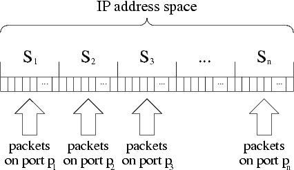
Figure 1: The first stage of the attack.
Second Stage
The second stage of the attack repeats until the attack is complete.
In each iteration, we take the k intervals that currently remain,
call them R1, . . . Rk, and distribute our n ports among them,
assigning n/k to each. Then for each i in
{1, . . . k}, we do the following.
Divide Ri into n/k +1 subintervals,
as shown in Figure 2. We send a packet
on the first port assigned to this interval to each address in the
first subinterval, a packet on the second port to each address in the
second subinterval, and so on, finally sending a packet on the last
port to each address in the n/kth subinterval, which is the
next to last. We do not send anything to the addresses in the last
subinterval. We will instead deduce the number of monitored addresses
in that subinterval from the number of monitored addresses in the
other subintervals. After this process is completed for each of the
subintervals of each of the remaining intervals, we wait two hours and
retrieve a report. Now we are given the number of monitored addresses
in each of the subintervals except the last in each interval. We then
determine the number in the last subinterval of each interval by
subtracting the number found in the other subintervals from the total
known to be in that interval. At this point, empty subintervals may
again be discarded. Additionally, subintervals with a number of
monitored addresses equal to the number of address in the subinterval
may be discarded after adding their addresses to a list of monitored
addresses found so far. The remaining subintervals, which contain both
monitored addresses and unmonitored addresses, may now be considered
our new set of remaining intervals R'1, . . .
R'k, and we repeat the procedure.
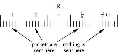
Figure 2: Subdividing an interval Ri within the second
stage of the attack.
By continuing to subdivide intervals until each is broken into pieces
full of monitored addresses or without any monitored addresses, we
eventually check every IP address and produce a list of all that are
monitored. This process may be visualized as in
Figure 3, which gives an example of the algorithm
being applied to a small number of addresses. The first row of boxes
in the figure represent the initial list of IP addresses to be
checked, with monitored addresses shaded. Six ports are used to probe
these addresses, giving the numbers of monitored addresses above the
row. Three intervals are ruled out as being empty, and the other three
are passed to the second stage of the algorithm. The six ports are
used in the first iteration of the second stage to eliminate three
subregions (of two addresses each), and mark one subregion as filled
with monitored addresses. The second iteration of the second stage of
the algorithm terminates, having marked all addresses as either
monitored or unmonitored. One caveat of the algorithm that did not
arise in this example is that the number of remaining intervals at
some stage may exceed n, the number of available ports. In this case
it is not possible to divide all those intervals into subintervals in
one time period, since at least one port is needed to probe each
interval. When this cases arises, we simply select n of the
subintervals to probe, and save the other subintervals for the next
iteration.
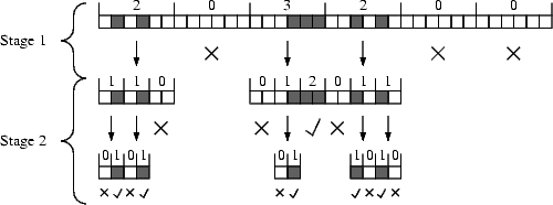
Figure 3: Illustration of the sensor probing algorithm.
4.3 Dealing With Noise
We now turn to a practical problem that must be addressed if the
attack is to function correctly. The problem is that sources other
than the attacker may also be sending packets to monitored addresses
with the same destination ports that the algorithm is using, inflating
the number of targets reported. This can cause the algorithm to
produce both false positives and false negatives. This background
activity may be considered noise that obscures the signal the attacker
needs to read from the port reports. For a large number of ports,
however, this noise is typically quite low, as shown by Table 3. Each row in the table gives the
approximate number of ports that typically have less than the given
number of reports. The numbers were produced by recording which ports
had less than the given number of reports every day over a period of
ten consecutive days.
| ports | reports |
| 561 | <= 5 |
| 19,364 | <= 10 |
| 41,357 | <= 15 |
| 51,959 | <= 20 |
| 56,305 | <= 25 |
Table 3: Ports with little activity.
A simple technique allows the algorithm to tolerate a certain amount
of noise at the expense of sending more packets. If there are
normally, say, less than five reports for a given port p, we may use
port p to perform probes in our algorithm by sending five packets
whenever we would have otherwise sent one. Then when reviewing the
published port report, we simply divide the number of reports by five
and round down to the nearest integer to obtain the actual number of
submitting hosts we hit. We subsequently refer to this practice as
using a "report noise cancellation factor" of five. Thus by sending
five times as many packets, we may ensure that the algorithm will
function correctly if the noise on that port is less than five
reports. Similarly, by using a report noise cancellation factor of
ten, we may ensure the algorithm operates correctly when the noise is
less than ten reports. By examining past port reports, we may
determine the least active ports and the number of packets necessary
to obtain accurate results when using them to perform probes.
4.4 Improvements
False Positives and Negatives
The attack may potentially be sped up by allowing some errors to
occur. If it is acceptable to the attacker to merely find some
superset of (i.e., a set containing) the set of hosts submitting their
logs to the ISC, they may simply alter the termination conditions in
the algorithm. Rather than continuing to subdivide intervals until
they are determined to consist entirely of either monitored or
unmonitored addresses, the attacker may mark all addresses in an
interval as monitored and discontinue work on the interval when it is
determined to consist of at least, say, 10 percent monitored
addresses. In this way, when the algorithm completes, at most 90
percent of addresses determined to be monitored are false positives.
Even though that is a large amount of error, the vast majority of the
addresses on the Internet would remain available for the attacker to
attempt to compromise, free from the fear of being detected by the
ISC. Alternatively, if the attacker is willing to accept some false
negatives (i.e., find a subset of the hosts participating in the
network), they may discard an interval if the fraction of the
addresses that are monitored within it is less than a certain
threshold, again speeding up the attack. In
Section 5 we provide quantitative results on the
speedup provided by these techniques in the case of mapping the ISC.
Using Multiple Source Addresses
Speed improvements may also be obtained by taking advantage of the
sources field of the port reports. By spoofing source IP addresses
while sending out probes, an attacker may encode additional
information discernible in this field. If in the course of probing an
interval of addresses with a single port, the attacker sends multiple
packets to each address from various numbers of source IP addresses
and takes note of the number of sources reported, they may learn
something about the distribution of monitored addresses within the
interval in addition to the number of monitored addresses. The
following is a method for accomplishing this.
Multiple Source Technique
Before probing an interval of addresses on some port, we further
divide the interval into some number of pieces k, hereafter referred
to as the "multiple source factor." To the addresses in the first
piece, we send packets from a single source. To each of the addresses
in the second piece, we send packets from two sources. For the third
piece, we send packets from four source addresses to each address. In
general, we send packets from 2i-1 source addresses to each
address in the ith piece. Note that we already are sending multiple
packets to each address in order to deal with the noise described in
Section 4.3. If 2k-1 is less than or equal to the
report noise cancellation factor, then we can employ this technique
without sending any more packets; otherwise, more bandwidth is
required to send all 2k-1 packets to each address.
When the port report is received, we may determine whether any of the
pieces lacked monitored addresses by considering the number of sources
reported. For example, suppose k = 3 (i.e., we divide our interval
into three pieces) and five sources are reported. Then we know that
there are monitored addresses in the first and third intervals, and
that there are no monitored addresses in the second interval. This
additional information increases the efficiency of the probing
algorithm by often reducing the size of the intervals that need to be
considered in the next iteration, at the expense of potentially
increasing the bandwidth usage. Of course, this technique is only
useful to a limited degree, due to the exponential increase in the
number of packets necessary to use it more extensively. Depending on
the level of noise on the port, using a multiple source factor of two
or three achieves an improvement in probing efficiency with little to
no increase in the bandwidth requirements.
Noise
In order for this technique to perform accurately, we must deal with
noise appearing in the sources field of the port reports in addition
to the reports field. If even a single source address other than those
spoofed by the attacker is counted in the reported number of sources,
the attacker will have a completely inaccurate picture of which pieces
are empty. This problem may be solved in a manner similar to the
method for tolerating noise in the number of reports. Rather than
sending sets of packets with 1, 2, 4, . . .
and 2k-1
different source addresses to the k pieces, we may use 1m, 2m, 4m, . . .
and 2k-1m sources, where m is a positive integer
hereafter referred to as the "source noise cancellation factor."
Then the reported number of sources may be divided by m and rounded
down, ensuring accurate results if the noise in the number of sources
was less than m. For example, if a particular port normally has less
than three sources reported (when the attacker is not carrying out
their attack) and the attacker is dividing each interval into four
pieces, they may send sets of packets with 3,6,12, and 24 sources.
If seventeen sources are then reported, they divide by three and round
down to obtain five, the sum of one and four. The attacker may then
conclude that the second and fourth intervals have no monitored
addresses, and that the first and third intervals do have monitored
addresses.
Egress Filtering There is another practical concern
relating to this technique, and that is egress filtering of IP packets
with spoofed sources. The careful attacker should be able to avoid
running into any problems with this by selecting source addresses
similar to actual ones that are then likely to be valid addresses
within the same network. Not many such addresses are needed (since
this technique will likely only be employed to a limited degree for
the aforementioned reasons of bandwidth), and it is a simple task to
verify whether packets with a given spoofed address will be filtered
before leaving the network. All that is necessary is to send one to an
available machine outside the network and see if it arrives.
5 Simulation of the Attack
In the following section we describe the results of several simulated
probe response attacks on the ISC, assuming the set of ISC sensor
locations as well as various other possible sets of sensor locations.
For each attack, we detail the results including the time required and
the number of packets sent, along with a description of how the attack
progresses under various levels of resources and with optimizations to
our algorithm.
In the first scenario, we determine the exact set of monitored
addresses. While this attack is the most accurate, it is also the most
time consuming. Depending on the intentions of the attacker (see
Section 5.6), it may not be necessary to find the exact
set of monitored addresses. Thus, we also simulate finding a superset
and a subset of the monitored addresses. These scenarios may be more
practically useful since they require less time and resources.
In each case, we examine the interaction between the accuracy, time,
and resources necessary to undertake our attack. We demonstrate that
the proposed attack is feasible with limited resources and under time
constraints, and discuss the impact on the integrity of the sensor
network reports. Since an attacker can obtain an accurate map of the
sensors in less than a week, the integrity of the sensor network
reports is at risk. Section 6 discusses how to
apply the algorithm using reports from other sensor networks, and
Section 7 discusses possible countermeasures
that sensor networks can use to improve their vulnerability to such
attacks.
5.1 Adversarial Models
Available Bandwidth
In order to examine a broad range of scenarios, we provide the results
of simulations under three distinct adversarial models, the primary
difference between models being the resources of the attacker. Our
first attacker has 1.544 Mbps of upload bandwidth, equivalent to a T1
line and hereafter will be referred to as the T1 attacker. Our second
attacker has significantly more upload bandwidth, 38.4 Mbps, and
hereafter will be referred to as the fractional T3 attacker or, for
brevity, the T3 attacker. Finally, we examine the rate at which an
attacker with 384 Mbps of bandwidth could complete our attack. This
adversary will be referred to as the OC6 attacker.
While each attacker is denoted by a specific Internet connection, our
algorithm is not dependent upon a particular Internet connection or
attacker configuration. Our algorithm can be executed on a distributed
collection of machines or a single machine, with the time required to
complete our attack dependent only on the aggregate upload bandwidth.
Neither the number of machines nor their specific configurations are
important as long as they can be coordinated to act in unison. In
addition, because our attack does not require a response to be
received from a probe or any significant amount of state to be
maintained, we can ignore download bandwidth, network latency, and
computing resources.
Botnets
One potential way to acquire the necessary bandwidth is to use a
"botnet," or collection of compromised machines acting in unison.
The technology required to coordinate such a collection of machines
for a probe response attack is currently available and is under some
estimations commonly used. The most ubiquitous families of botnet
software are reported to be Gaobot, Randex, and Spybot. The required
upload bandwidth for the T1 attacker could easily be achieved by a
dozen cable modems, a very small botnet. Similarly, the upload
bandwidth for the fractional T3 attacker and the OC6 attacker could be
achieved by using around 250 and 2,500 cable modems, respectively.
Botnets of these scales are not uncommon [37].
It should be noted that the bandwidth required for the swift
completion of the attack varies widely based upon the noise
cancellation factors and the multiple source factor. In all of our
attack scenarios, we have configured the parameters of our algorithm
to best match the resources of the attacker, resulting in a near
optimal outcome for each attacker. Since the only factors that affect
the time required for our attack to complete are the upload bandwidth
and parameters to the algorithm, it is reasonably easy to find a near
optimal set of parameters for any given bandwidth. In addition, the
number of ports that have sufficiently low noise to be used in our
attack can easily be calculated from past port reports and is found to
remain steady throughout the duration of the attack.
Variation in Performance
Each of our attackers is representative of a class of adversaries
ranging from the most basic attacker with a dozen machines to a
sophisticated and resourceful group with thousands of machines at
their command. Using these classes of attackers, we show the tradeoffs
between accuracy, time, and resources while providing concrete results
including the time required to complete the attack and the rate at
which the attack progresses.
What may not be immediately obvious is the fact that almost any level
of resources is sufficient to map the addresses monitored by a log
collection and analysis center in a few months. For instance, while
not a likely case, an attacker equipped only with a DSL line could
find the exact set of addresses monitored by the ISC in under four
months. Log collection projects with fewer participants than the ISC
could be mapped in even less time.
5.2 Finding the Set of Monitored Addresses
First, we detail the results of our simulation of the fully accurate
attack, which finds the exact set of monitored addresses. Two useful
statistics that will help us to explain the specifics of an attack are
the number of probes sent and the fraction of monitored addresses
known at a particular time. We explain the significance of each of
these statistics and then use them to highlight similarities and
differences in the simulations under different adversarial models.
Number of Probes Sent
As previously explained in Section 4.2, our attack
utilizes repeated probing of IP addresses with SYN packets. Since we
must probe approximately 2.1 billion addresses with at least one
packet each, the number of packets sent by an attack is significant.
While the specifics vary based on the optimizations used, when finding
the exact set of monitored addresses, our algorithm may send from nine
billion to twenty seven billion SYN packets over a several day to
several week period. As a result of this hefty requirement, our three
attackers, with their widely different upload bandwidths, are able to
complete the attack in widely differing times. For instance, the time
required to find the set of monitored addresses exactly ranges from
around 3 days for the OC6 attacker to approximately 34 days for the T1
attacker. While the time required to complete an attack is not
directly proportional to the number of probes sent, as upload
bandwidth increases, the time required to complete an attack
monotonically decreases.
 |
 |
 |
| (a) Packets sent by T1 adversary. |
(b) Packets sent by fractional T3 adversary. |
(c) Packets sent by OC6 adversary. |
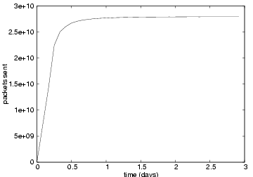
Figure 4: Number of packets sent for each attack simulation.
Figure 4 shows the specific number of packets
sent per attacker and the rate at which packets are sent when finding
the exact set of monitored addresses. The bend in the curve represents
the point at which the attacker's bandwidth is sufficient to send all
the packets required for a particular two hour interval within the
same two hour interval. Before the bend, the attacker's progress is
limited by the rate at which they can send out packets. This period
generally corresponds to the first stage of the attack, that is, the
initial probing of the entire non-bogon address space. The bandwidth
used in this stage accounts for the majority of the total bandwidth
used, as large portions of the address space are ruled out in this
first pass.
After the bend, the attacker's progress is limited by the two hour
wait between sending a set of probes and checking the corresponding
port reports. This situation is generally the case throughout most of
the iterations of the second stage of the algorithm. For the remainder
of our analysis, we will focus on the second statistic, the fraction
of monitored addresses known at a particular time.
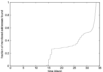
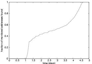
Attack Progress
Figure 5 shows the fraction of monitored
addresses that are known throughout the execution of the attack for
each of our three specific simulations. While in each case the end
result is always the same, the time required and the rate at which
addresses are discovered, a statistic we call the attack progress,
varies widely. One may notice that the lines in
Figure 5 are similar in shape. This is a
result of similarities in the sizes of intervals used in the algorithm
and the particular distribution of monitored addresses in IP address
space. Discussion of this distribution of addresses appears in
Section 5.5. We will continue to use the attack
progress statistic throughout our analysis as a way to provide insight
into the specifics of our algorithm.
 |
 |
 |
| (a) T1 adversary progress. |
(b) T3 adversary progress. |
(c) OC6 adversary progress. |
Figure 5: The attacker's progress in discovering monitored addresses.
T1 Attacker Analysis
When bandwidth is highly limited as in the case of the T1 attacker,
the number of packets sent in the first stage of the attack and the
first several iterations of the second stage are the primary time
constraint. As a result, it makes sense to reduce the number of
packets sent by using ports with less noise and avoiding the use of
the multiple source technique. This in turn allows an attacker to use
a lower report noise cancellation factor, however this also results in
fewer available ports. We have found that when one doubles the number
of ports available for use by the attacker, they in turn reduce the
number of intervals required to complete the attack by a factor of
two. However, this is only beneficial when the attacker is able to
send the number of packets required in each interval. Since this is
not always possible in the case of low bandwidth attackers, it makes
sense to reduce the number of packets required and in turn use fewer
ports for the attack. Specific details for a near optimal set of
parameters for the T1 attacker and other low bandwidth attackers
follow.
When simulating our algorithm with an upload bandwidth equivalent to
that of a T1, we determined that a report noise cancellation factor of
two and avoiding the use of the multiple source technique was one of
the best options. As a result of the T1 attacker's inability to send a
sufficient amount of packets in the first stage of the algorithm and
the majority of the iterations of the second stage, the T1 attack
takes significantly more time to run than the T3 attack or OC6 attack.
A T1 line can only send roughly 28 million SYN packets in a two hour
interval, thus the T1 attacker requires several days to run the first
stage of the attack. Similar results follow for most of the iterations
of the second stage of the attack. This slow progress results in the
complete lack of monitored addresses found within the first 15 days of
the attack. However, after the T1 attacker is able to send the number
of probes required for a particular interval, which happens around day
27, the remaining 60 percent of monitored addresses are found in only
7 days. In the end, the T1 attacker requires 33 days and 17 hours and
the transmission of approximately 9.5 billion packets to find the
exact set of monitored addresses by the ISC.
T3 Attacker Analysis
As can be seen from Figure 4(b), the T3
attacker is able to quickly send the number of probes required by the
first stage of the attack and the following iterations of the second
stage. With a maximum upload throughput of about 626 million SYN
packets in a two hour period, the T3 attacker can complete the first
stage of the attack in 23 hours. Since the first stage of the attack
requires over 8 billion packets, the T3 attacker has already sent the
majority of the 14 billion packets required for the entire attack and
is well ahead of where the T1 attacker was at the same time.
By the end of the 30th hour, the T3 attacker has already found about
30 percent of the monitored addresses and is able to send the number
of probes required by all successive intervals within the interval
itself. Correspondingly, the remaining 65 percent of monitored
addresses are found in the following three days. These results were
achieved with a report noise cancellation factor of two, a multiple
source factor of two, and a source noise cancellation factor of two.
The time required for the completion of this simulated attack was 4
days and 16 hours. This represents greater than a factor of 7
reduction from the T1 attacker's 33 days and 17 hours, however this
was obtained with an almost 2,500 percent increase in bandwidth.
OC6 Attacker Analysis
While the OC6 attacker has sufficient upload bandwidth to undertake a
faster attack than both other adversaries, the difference between the
time required for the T3 adversary and the OC6 adversary is only a
fraction of the difference between the T1 and T3 adversaries. Even
though the OC6 attacker has 10 times the bandwidth of the T3 attacker,
an increase in the multiple source factor (the only remaining
optimization possible) is not feasible because of the corresponding
exponential increase in the number of probes required. We determined
that a near optimal set of parameters for the OC6 attacker was a
multiple source factor of two with a source based noise cancellation
factor of four and a report noise cancellation factor of eight. This
not only balances the number of packets required by the multiple
source technique with the number required by the report noise
cancellation factor, but also allows for 25 percent more ports to be
used for the OC6 attack than were used for the T3 attack.
Under these parameters, the OC6 attacker can find the exact set of
monitored addresses to the ISC in 70 hours. If we were to continue
considering increasing bandwidths, we would continue to notice
diminishing marginal returns. This is a result of the fact that the
only remaining optimization possible is the usage of the multiple
source technique, and, as previously stated, this results in an
exponential increase in the number of packets sent while only reducing
the time required to complete our attack by a few hours.
| type of mapping |
bandwidth available |
data sent |
false positives |
false negatives |
correctly mapped addresses |
time to map |
| exact |
OC6 |
1,300GB |
0 |
0 |
687,340 |
2 days, 22 hours |
| exact |
T3 |
687GB |
0 |
0 |
687,340 |
4 days, 16 hours |
| exact |
T1 |
440GB |
0 |
0 |
687,340 |
33 days, 17 hours |
| superset |
T3 |
683GB |
3,461,718 |
0 |
687,340 |
3 days, 6 hours |
| subset |
T1 |
206GB |
0 |
182,705 |
504,635 |
15 days, 18 hours |
Table 4: Time to map sensor locations. (ISC sensor distribution)
5.3 Finding a Superset
By setting a configurable threshold in our algorithm (see
Section 4.4), an attacker is capable of accepting
some number of false positives, while avoiding false negatives. As a
result, an attacker that is interested in simply avoiding detection
may further improve upon the results given above by finding a superset
of the monitored addresses. We detail the results of such an attack
with the T3 adversarial model.
In order to compare with previous results, we use the same parameters
as were used when the T3 adversary found the exact set of monitored
addresses, except in this case, we specify a maximum percentage of
false positives to allow on a per interval basis. With a maximum false
positive rate of .94 (i.e., the number of possible false positives
over the total number of IP addresses), a report noise cancellation
factor of four, a multiple source factor of two, and a source noise
cancellation factor of two, we are able to reduce the runtime of our
attack from 112 hours to 78 hours. However, this reduction in time
requires us to accept around 3.5 million false positives along with
our set of monitored addresses. Allowing these false positives had
little effect on the number of probes. It was reduced by less than one
percent. This phenomena occurs because the final iterations of the
second stage of the algorithm require fewer and fewer packets to probe
the small intervals that remain. This fact can also be seen in
Figure 4, where the lines flatten out near the
end of the attack. Although the modest improvement in time in this
case is likely not worth the decrease in accuracy, in other cases of
probe response mapping attacks accepting false positives may be more
useful.
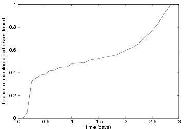
5.4 Finding a Subset
Having examined the cases of finding an exact set and finding a
superset, we now examine a situation where an attacker may be
interested in finding a subset of the monitored addresses. While an
attacker with a T3 or OC6 may attempt to find the exact set of
monitored addresses, an impatient attacker or an attacker with less
resources, such as the T1 attacker, may be content with finding a
subset of the monitored addresses in a reduced amount of time. By
allowing false negatives, an attacker may reduce the time and
bandwidth necessary to undertake the attack, but still discover a
large number of monitored IP addresses. An attacker who is interested
in flooding the monitored addresses with spurious activity rather than
avoiding them may be especially interested in allowing false
negatives. In addition to saving time, an attacker finding a subset
may potentially avoid detection of their attack by sending
significantly fewer probes overall.
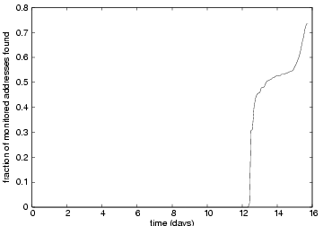
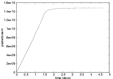
Figure 6: The T1 adversary finding a subset of the monitored addresses.
Since the difference between the time required to find the exact set
of monitored addresses and the time required to find a subset of
monitored addresses is less pronounced at high bandwidths, we only
detail the results of finding a subset with the T1 adversary. Once
again we use the same parameters that were used when the T1 adversary
found the exact set of monitored addresses, except this time we set
the maximum false negative rate (i.e., the number of possible false
negatives over the total number of IP addresses). With a report noise
cancellation factor of two, a single source address, and a maximum
false negative rate of .001, we are able to reduce the runtime of our
attack from 33 days and 17 hours to 15 days and 18 hours. In addition,
we reduce the number of probes sent from around 9.5 billion to 4.4
billion, a reduction of over 50 percent. However, these reductions
come at the cost of missing 26 percent of the sensors. The progress of
this scenario is depicted in Figure 6.
5.5 General Sets of Monitored Addresses
The preceding scenarios (summarized in
Table 4) demonstrate that a probe response
attack is practical for mapping the IP addresses monitored by the ISC.
They do not, however, reveal how dependent the running time of the
attack is on this particular set of addresses. A key factor that
determines the difficulty of mapping the addresses of a sensor
network is the extent to which the sensors are clustered together in the
space of IP addresses. As mentioned in Section 4.1,
the more the addresses are clustered together, the more quickly they
may be mapped. This fact is easily seen in Figure 3.
To determine how well the algorithm works more generally against
various possible sets of sensor IP addresses, we generated random sets
of IP addresses based on a model of the clustering. More specifically,
the sizes of "clusters," or sets of sequential sensor addresses,
were drawn from a Pareto distribution, and the sizes of the gaps in address space between them were
drawn from an exponential distribution. With the parameters of the two
distributions set to fit the actual addresses of the ISC, the times to
map various random sets of IP addresses are similar to the times
reported in Table 4. By varying the parameters
of the distributions, sets of IP addresses with various average
cluster sizes were produced while holding the total number of sensors
roughly constant at 680,000, the approximate number in the ISC set.
For average cluster sizes of 10 or more, the attack typically takes
just over two days to complete under the T3 attacker model previously
described (compared to the 4 days, 16 hours to complete the attack for
the actual ISC). For smaller average cluster sizes, the running time
increases. Below the average cluster size of the ISC ( ~ 1.9),
typical running times increase rapidly, with about eight days (about
twice the time to map the ISC sensors) at average clusters size of
about 1.6. Note that smaller sensor networks are faster to map; the
ISC network is among the most challenging networks to map due to its
large number of sensors with widely scattered IP addresses.
As an extreme case, a number of simulations were also run on sets of
IP addresses that possessed no special clustering, again using the T3
attacker model. Specifically, the sets were produced by picking one IP
address after another, always picking each of the remaining ones with
equal probability. This can be considered a worst case scenario, since
any real life sensor network is likely to display some degree of
clustering in its set of addresses. The attack remained quite feasible
in this case, taking between two to three times as long as in the ISC
case when working on a set of addresses of the same size. This
scenario was tested for sets of IP addresses of various sizes. The
running time ranged linearly from about 3 days to map 100,000
addresses to about 21 days to map 2,000,000.
5.6 Summary and Consequences
Perhaps the most interesting results of the simulations using the
addresses monitored by the ISC presented in
Table 4 are the cases of discovering the exact
set of monitored addresses in about a month with low bandwidth and in
about three days with high bandwidth. The consequences of a malicious
user successfully mapping a set of sensors are severe. Armed with a
list of the IP addresses monitored by a log collection and analysis
center, an attacker could avoid the monitored addresses in any future
suspicious activities (such as port scanning). It would even be
possible to include the list in any worms they released, allowing the
worms to avoid scanning any monitored addresses as they spread. Such
attacks would go undetected (at least by the analysis center in
question). Since organizations such as the ISC are often the first to
discover the spread of new worms, a worm avoiding the addresses they
monitor may go undetected for a long time. Another technique an
attacker armed with a list of monitored addresses might employ is to
flood monitored addresses with activity, causing valid alerts to be
lost in the noise.
The most important thing to realize when considering the consequences
of an adversary having obtained a list of monitored addresses is that
the damage done to the distributed monitoring effort is essentially
permanent. If the list were publicly released, future alerts arising
from those monitored addresses could not be considered an accurate
picture of the malicious activities occurring within the Internet.
Since organizations cannot easily change the IP addresses available to
them, and since distributed monitoring projects cannot arbitrarily
select who will participate, accumulating a new set of secretly
monitored IP addresses could be an extremely time consuming task.
6 Generalizing the Attack
We return now to the fact that our example algorithm for mapping a set
of sensors is highly tailored to our example, the ISC, and its port
reports. It is certainly conceivable that some change may be made to
the way this information is reported that will confound the algorithm
as it is given. But given such a change, how may we be sure that all
attacks similar to the one given may be prevented? To address this
problem, we need to understand what essentially allows the example
attack to work.
6.1 Covert Channels in Reports
By sending probes with different destination ports to different IP
addresses and considering which ports have activity reported, the
attacker is able to gain some information about the set of IP
addresses that could have possibly received the probes. In this way,
the destination port appearing in a packet sent out and later in the
port reports is used by the attacker as a covert channel [38]
in a message to themselves. The covert channel stores partial
information about the IP address to which the probe was directed.
Similarly, (and here we are considering the "probe" to be all the
packets sent to a particular address in a single round of the second
stage of the algorithm) we see that the number of packets sent and the
number of distinct source IP addresses they contain are covert
channels that may be used to store additional information.
Viewed in this light, it is clear that many possible fields of
information one may imagine appearing in the reports published by a
sensor analysis center are suitable for use as covert channels in
probe response attacks. Characteristics of attacks or probes that may
be reported include the following.
- Time / date
- Source IP
- Source network
- Source port
- Destination network
- Destination port
- Protocol (TCP or UDP)
- Packet length
- Captured payload data or signature
Our case study attack uses the time a probe was sent out, its
destination port, and its set of source IP addresses as the covert
channels. The possibility of characteristics of packets being used as
a covert channel has been previously mentioned by Xu, et
al. [28].
6.2 Other Internet Sensor Networks
To demonstrate the generality of our algorithm, we outline how an
attacker could map the Symantec DeepSight Analyzer and the
myNetWatchman sensor network. Table 5 summarizes the
essential mapping information for Symantec DeepSight, myNetWatchman,
ISC, and the modeled ISC distribution.
Symantec DeepSight
Besides the SANS Internet Storm Center, the largest Internet sensor
network that publicly displays statistics is Symantec's DeepSight
network. Designed much like the ISC, DeepSight provides a sensor client
called the DeepSight Extractor which, once installed, forwards
firewall and IDS logs from a monitored address to a central log
analysis center named the DeepSight Analyzer. The DeepSight Analyzer
then produces summaries and statistics related to the specific
security events seen by the particular client. After installing the
client software, a particular client can log into the DeepSight system
and view statistics concerning the attacks seen in their own logs.
This differentiates the reports of the DeepSight system from those of the
ISC since the DeepSight system does not provide a global report of the
activity sensed by all clients, but rather primarily a view of
the events seen by a specific client.
Despite the fact that DeepSight primarily provides information
concerning security events seen in a particular client's logs, they
are still vulnerable to a probe response attack. In order to see how
an attacker would map the DeepSight network, we first need to analyze
the output provided by DeepSight. DeepSight provides each client with
a detailed report of the attacks seen in their logs including the time
and date, source IP address, source port, destination port, and the
number of other clients affected by a particular attack. Each report
listed contains roughly forty-two to seventy-four bits usable to the
attacker as a covert channel. There are about ten in the time field,
sixteen in each port field, and zero to thirty-two in the source
address field (depending on whether the attacker needs to worry about
egress filtering when spoofing source addresses and to what extent if
so). With this information, an attacker could map DeepSight with a few
simple modifications to our algorithm.
First, instead of using strictly the time, destination port, and set
of source IP addresses to encode the destination address as in the ISC
example, an attacker could encode the destination address in the
source IP, destination port, source port, and time fields. Since the
source IP address alone provides sufficient space to encode the
destination IP address, encoding information in the source and
destination ports and time field is not strictly necessary but could
be useful for noise reduction purposes or if egress filtering is an
issue. Second, for each unique combination of fields which the
attacker uses to encode the destination address, the attacker will
have to submit a log to DeepSight which contains these specific
fields. This will allow an attacker to view the required response
statistics for that probe in the DeepSight system, most importantly,
the number of other clients that received the probe. Using these two
simple modifications to our example algorithm, an attacker should be
able to encode sufficient information in each probe such that the
DeepSight network could be mapped in a single pass of probes.
myNetWatchman
Another important example of an Internet Sensor network that displays
public statistics is myNetWatchman. The myNetWatchman sensor network
groups the events of the past hour by source IP and lists them in the
"Largest Incidents: Last Hour" report. For each source IP, this
report lists the time, target subnet, source port, and destination
port of the most recent event. The addresses monitored by
myNetWatchman could be discovered in a single pass of probes using
this or other available reports.
| network |
bandwidth |
probes sent |
time to map |
| DeepSight |
- |
2.1 billion |
single pass of probes |
| myNetWatchman |
- |
2.1 billion |
single pass of probes |
| SANS ISC |
T3 |
14 billion |
4 days 16 hours |
| Modeled ISC |
T3 |
20 billion |
6 days 6 hours |
Table 5: Essential mapping results.
6.3 Other Types of Reports
Necessity of Event Counts
It is important to note that it is not even strictly necessary for the
reports to include the number of events matching some criteria, but
only their presence or absence. In terms of the algorithm of the
example attack as given in Section 4.2, it would no
longer be possible to avoid sending probes to the last addresses in
each interval. Instead, probes would always have to be sent to all the
subintervals. Also, a different scheme would be needed to overcome the
noise problem described in Section 4.3 (probably sending
several probes to an interval and only marking it as containing a
submitting address if the corresponding port consistently reports
activity), but the attack could still be made to work.
Top Lists
One type of report commonly produced by log analysis centers is the
"top list" or "hot list," essentially a list of the most common
values of a field within the reports. For example, the "Top 10
Ports" report produced by the ISC is a list of the most frequently
occurring destination ports among events in the past day. The number
of values listed on the report may be a fixed number (in this case
ten), or it may vary as in the case of reports that list all values
occurring more often than some threshold. Such top list reports tend
to be less useful for conducting probe response attacks for a couple
reasons. Reports with a fixed length typically report very little
total information. A probe response attack based only on the ISC "Top
10 Ports" report would take far too long to be feasible. Also, it may
be necessary to generate a very large amount of activity to appear on
a top list, also making the attack infeasible. Nevertheless, other
such reports still merit a critical look to determine if they may be
sufficient to launch a probe response attack. Such reports are likely
to be more dangerous if they may be requested for various criteria
(e.g., top ten ports used in attacks directed at a particular subnet
rather than just top ten ports).
7 Countermeasures
7.1 Current Methods
Several methods are in use or have been proposed for preventing
information published in reports from being misused.
Hashing and Encryption
One common technique is to hash some or all of the above fields.
However, in general this does not impair the attack as the attacker
(having generated the original probes) has a list of the possible
preimages, which allows for an efficient dictionary attack. However,
encrypting a field with a key not publicly available (or using a keyed
hash such as HMAC-SHA1) would prevent the use of that field in a
covert channel. Unfortunately, it would also prevent nearly any use of
the information in that field by those who read the published reports
for legitimate purposes. Prefix-preserving
permutations [28] have been proposed a method for
obscuring source IP addresses while still allowing useful analysis to
take place. Obscuring source IP addresses with encryption (whether or
not it is prefix-preserving) does not, however, prevent probe response
attacks, as any of the other characteristics listed in
Section 6.1 may be used.
Bloom Filters
The Bloom filters popular for storing a set of source IP
addresses [25,7] suffer from similar problems. In
general, a Bloom filter storing a set of IP addresses is in fact safe
from dictionary attacks due to the false positive feature of Bloom
filters. Even with a relatively low rate of false positives, say 0.1
percent, the number of false positives resulting from checking all
non-bogon IP addresses against the filter is on the order of two
million (likely much more than the number of addresses actually stored
in the filter). However, Bloom filters do not stand up to the
iterations of a probe response attack. As an example, suppose some
analysis center receives logs from monitored addresses and at the end
of each time interval publishes a Bloom filter containing the source
addresses observed. Sending probes to all non-bogon addresses with the
destination address encoded in the source address, then checking for
those addresses in the resulting Bloom filter would produce on the
order of two million false positives (along with the true positives).
Sending a second set of probes to all positives would reduce the
number of false positives to about two thousand, and after re-probing
those positives, approximately two false positives would remain. One
more round would likely eliminate all remaining false positives, an
accurate set of monitored addresses having been determined in four
probe response iterations. There are of course the additional
complications of noise and egress filtering, but this example
illustrates that the number of false positives decreases exponentially
with respect to the number of iterations of the probe response attack.
7.2 Information Limiting
Private Reports
The most immediately apparent way to prevent attackers from mapping
the locations of the sensors is to limit the information published in
the reports. The most heavy handed implementation of this strategy is
to eliminate public reports entirely and only provide reports to
persons and organizations that can be trusted to not attempt to map
the sensor locations and not disclose reports to others. Clearly, such
an approach severely limits the utility of the network. Only a select
few obtain any benefit at all from the information collected and the
analysis performed on that information.
Top Lists
The strategy of producing no public reports is probably overly
cautious. It is likely possible to publish a variety of the "top
list" style reports described in Section 6.3 without
disclosing enough information to enable fast probe response attacks,
provided some care is used. However, such lists do not provide
anything approaching a complete picture of the activity within the
Internet. In particular, publishing only top list style reports allows
attackers to ensure their continued secrecy by intentionally limiting
their activity to the extent necessary to stay off the lists.
Query Limiting
Alternatively, a log analysis center may provide full public reports
or queries of all kinds, but limit the rate at which they can be
downloaded. This may be accomplished by requiring payment for each
report downloaded. The payment may be monetary, or it may take a more
virtual form. Such virtual payments may be the computational effort
required to solve a puzzle or the human interaction necessary to
answer a CAPTCHA [39]. These transactional networks are
similar to those proposed by researchers who are attempting to stem
the flood of spam email. This may be used in conjunction with
providing complete reports free of payment to any organizations that
are completely trusted.
Sampling
Another strategy in limiting the information available to an attacker
attempting to map the sensor locations is to sample the logs coming
into the analysis center before generating reports from them. For
example, the analysis center may discard every log it receives with
probability 4/5. Large scale phenomena such as worm
outbreaks and port scanning should remain clearly visible in the
reports [10], but a probe response attack would be more
difficult. The probability of a single probe sent by an attacker to a
monitored address resulting in a false negative would be
4/5; to reduce this, the attacker would need to send
multiple probes. If the attacker wished to reduce it to, say, 1
percent, they would need to send twenty probes. A twenty-fold increase
in bandwidth is substantial, and a large number of false negatives
would still likely result if the attacker attempted to map a network
with hundreds of thousands of monitored addresses in that manner. Of
course, this technique of sampling the incoming alerts does reduce the
useful information produced by the analysis center. It has an
advantage over the strategy of only publishing top list style reports,
however. In this case there is no way for an attacker to be certain
they will not appear in a report by limiting their activity. Even
small amounts of malicious activity have a chance of being reported.
7.3 Other Techniques
Scan Prevention
An additional countermeasure which effectively renders our current
algorithm useless is the widespread adoption of IPv6. With a search
space of 128 bits, IPv6 greatly reduces the feasibility of TCP/UDP
scanning and prevents the first stage of our attack from completing in
a reasonable amount of time. Mechanisms for reducing the search space
required for scanning in IPv6 such as exploiting dual-stacked
networks, compiling address lists, and mining DNS have been previously
addressed in [40]. While IPv6 is an effective
countermeasure, the widespread adoption of IPv6 is out of the control
of a sensor network and hence is an impractical countermeasure.
Delayed Reporting
By waiting to publish public reports for a period of time, an Internet
sensor network can force an attacker to expend more time and bandwidth
in mapping a network. To undertake a probe response attack in the face
of delayed reporting, an attacker has two primary options: either wait
to receive the responses from the most recent probes or continue
probing using a nonadaptive probe response algorithm. Nonadaptive
probe response algorithms do not rely on the responses of the previous
round's probes to select the next intervals to probe, rather they
continue probing and partitioning a likely larger search space than
necessary under the assumption that a report will be produced at some
point in time and that this report will allow for a much larger search
space reduction than a single round of probe responses would have.
However, since nonadaptive algorithms do not reduce the search space
after each round of probes, they require significantly more probes to
be sent and hence increase the bandwidth necessary for an attack to
complete. We defer a full discussion of nonadaptive probing to future
work. The other alternative of waiting for reports to be published is
likely only possible if the delay is small. Of course, if a network
can be probed in a single round then a waiting time of one week before
publishing reports is not an effective countermeasure. Hence, delayed
reporting should be used in conjunction with another technique which
reduces the amount of information leakage. It should also be noted
that the utility of a network designed to produce near real time
notifications of new attacks is greatly reduced by delayed reporting.
Eliminating Inadvertent Exposure
Our final countermeasure is more of a practical suggestion rather than
a general countermeasure. Internet sensor networks and log analysis
centers should avoid publishing information about the specific
distribution of addresses they monitor. A simple example should serve
to highlight the primary types of information that must be eliminated
from log analysis center descriptions. Take for example a log analysis
center that publicly provides their complete sensor distribution,
perhaps monitoring a single /8. In this case, we can simply probe all
/8's and wait for a single probe to show up in the statistics reported
by the sensor network. The singular fact that the log analysis center
monitors a /8 network provides us with enough information to reduce
the number of probes sent by our attack from several billion to 256!
Even more complicated distributions like those provided
in [20] should be eliminated as they provide very little
useful information and make the attacker's job much easier. It should
be noted that systems like honeypots, iSink, and network telescopes
which often monitor contiguous address space are particularly
vulnerable to this sort of inadvertent exposure.
8 Conclusion
In this paper we developed a general attack technique called probe
response, which is capable of determining the location of Internet
sensors that publicly display statistics. In addition, through the use
of the probe response algorithm, we demonstrated critical
vulnerabilities in several anonymization and privacy schemes currently
in use in Internet analysis centers. We simulated a probe response
attack on the SANS Internet Storm Center, as well as on various
distributions of sensor nodes that could occur in other sensor networks,
and were able to determine the set of monitored addresses within a
few days with limited resources. Finally, we
outlined the consequences of a successful mapping of Internet sensors,
alternative reporting schemes, and countermeasures that defend against
the attacks.
Our current mapping algorithm is an adaptive probe response algorithm
as each round depends on the output of the previous round. On-going
and future work includes developing and evaluating a nonadaptive
approach for efficiently mapping Internet sensor networks that
infrequently provide data sets or delay reports. Such networks include
the University of Michigan Internet Motion Sensor [19,20],
CAIDA [2], and iSink [10]. Another issue to be
investigated in future work is the effectiveness of proposed
countermeasures.
Acknowledgments
We would like to acknowledge Johannes Ullrich of the SANS Institute
for providing access to the DShield logs. We would also like to thank
Eric Bach for his valuable insights and pointers and the anonymous
reviewers for their suggestions. This work was supported in part by
the U.S. Army Research Laboratory and the U.S. Army Research Office
under grant number #DAAD19-01-1-0502. Jason Franklin performed this
research while on appointment as a U.S. Department of Homeland
Security (DHS) Scholar under the DHS Scholarship and Fellowship
Program.
References
- [1]
- The SANS Internet Storm Center,
https://isc.sans.org.
- [2]
- CAIDA, the Cooperative Association for Internet Data
Analysis,
https://www.caida.org.
- [3]
- Computer Emergency Response
Team. AirCERT. https://www.cert.org/kb/aircert/, 2003.
- [4]
- C. Zou, L. Gao, W. Gong, and D. Towsley. Monitoring and
Early Warning for Internet Worms. Proceedings of CCS'03,
October 2003.
- [5]
- The National Strategy to Secure Cyberspace,
https://www.securecyberspace.gov.
- [6]
- V. Yegneswaran, P. Barford, and S. Jha. Global
Intrusion Detection in the DOMINO Overlay System. Proceedings
of the 2004 Network and Distributed System Security Symposium (NDSS
2004), February 2004.
- [7]
- M. Locasto, J. Parekh, S. Stolfo, A. Keromytis, T.
Malkin, and V. Misra. Collaborative Distributed Intrusion Detection.
Tech Report CUCS-012-04, Department of Computer Science, Columbia
University, 2004.
- [8]
- N. Provos. Honeyd - a virtual honeypot daemon.
Proceedings of the 10th DFN-CERT Workshop, February 2003.
- [9]
- L. Spitzner. Know Your Enemy: Honeynets.
Honeynet Project,
https://project.honeynet.org/papers/honeynet.
- [10]
- V. Yegneswaran, P. Barford, and D. Plonka. On the
Design and Utility of Internet Sinks for Network Abuse Monitoring.
Proceedings of Symposium on Recent Advances in Intrusion
Detection (RAID), September 2003.
- [11]
- D. Moore. Network Telescopes: Observing Small or
Distant Security Events. Invited Presentation at the 11th
USENIX Security Symposium (SEC 02), August 2002.
- [12]
- V. Yegneswaran, P. Barford, and J. Ullrich.
Internet Intrusions: Global Characteristics and Prevalence.
Proceedings of ACM SIGMETRICS, June 2003.
- [13]
- R. Pang, V. Yegneswaran, P. Barford, V. Paxson, and
L. Peterson. Characteristics of Internet Background Radiation,
Proceedings of ACM SIGCOMM/USENIX Internet Measurement Conference,
October 2004.
- [14]
- H. Kim and B. Karp. Autograph: Toward Automated,
Distributed Worm Signature Detection. USENIX Security
Symposium, 2004.
- [15]
- C. Kreibich and J. Crowcroft. Honeycomb -
Creating Intrusion Detection Signatures Using Honeypots.
Proceedings of the IEEE Symposium on Security and Privacy, May
2004.
- [16]
- S. Singh, C. Estan, G. Varghese, and S. Savage.
The EarlyBird System for Real-time Detection of Unknown Worms.
Technical Report CS2003-0761, UCSD, August 2003.
- [17]
- Symantec DeepSight Threat Management System
Technology Brief
- [18]
- The myNetWatchman Project,
https://www.mynetwatchman.com.
- [19]
- The University of Michigan Motion Sensor,
https://ims.eecs.umich.edu.
- [20]
- M. Bailey, E. Cooke, F. Jahanian, J. Nazario, and
D. Watson. The Internet Motion Sensor: A Distributed Blackhole
Monitoring System. Proceedings of the 12th Annual Network and
Distributed System Security Symposium, February 2005.
- [21]
- D. Moore, C. Shannon, and J. Brown. Code-Red: A Case
Study on the spread and victims of an Internet worm.
Proceedings of the 2nd ACM Internet Measurement Workshop, pages
273-284. ACM Press, November 2002.
- [22]
- D. Moore, V. Paxson, S. Savage, C. Shannon,
S. Staniford, and N. Weaver. Inside the Slammer Worm. IEEE
Security and Privacy, 1(4):33-29, July 2003.
- [23]
- D. Moore, G. Voelker, and S. Savage. Inferring Internet
Denial-of-Service Activity. Proceedings of USENIX Security
Symposium, 2001.
- [24]
- B. Bloom. Space/Time Trade-Offs in Hash Coding With
Allowable Errors. Communications of the ACM, 1970. 13(7): p.
422-426.
- [25]
- P. Gross, J. Parekh, and G. Kaiser. Secure
"Selecticast" for Collaborative Intrusion Detection Systems.
Proceedings of the 3rd International Workshop on Distributed
Event-Based Systems (DEBS'04), May 2004.
- [26]
- A. Slagell, J. Wang, and W. Yurcik. Network Log
Anonymization: Application of Crypto-PAn to Cisco Netflows.
Proceedings of the Workshop on Secure Knowledge Management 2004,
September 2004.
- [27]
- G. Minshall. TCPdpriv: Program for Eliminating
Confidential Information from Traces. Ipsilon Networks, Inc.
https://ita.ee.lbl.gov/html/contrib/tcpdpriv.html
- [28]
- J. Xu, J. Fan, M. Ammar, and S. Moon.
Prefix-Preserving IP Address Anonymization: Measurement-based
Security Evaluation and a New Cryptography-based Scheme.
Proceedings of the 10th IEEE International Conference on Network
Protocols (ICNP'02), November 2002.
- [29]
- S. Staniford, V. Paxson, and N. Weaver. How
to 0wn the Internet in Your Spare Time. Proceedings of the 11th
USENIX Security Symposium, 2002.
- [30]
- P. Lincoln, P. Porras, and V. Shmatikov.
Privacy-Preserving Sharing and Correlation of Security Alerts.
Proceedings of the 13th USENIX Security Symposium, 2004.
- [31]
- A. Slagell and W. Yurcik. Sharing Computer Network Logs
for Security and Privacy: A Motivation for New Methodologies of
Anonymization. ACM Computing Research Repository (CoRR)
Technical Report 0409005, September 2004.
- [32]
- R. Pang and V. Paxson. A High-level Programming
Environment for Packet Trace Anonymization and Transformation.
Proceedings of SIGCOMM 2003, August 2003.
- [33]
- K. Carr and D. Duffy. Taking the Internet by
storm. CSOonline.com, April 2003.
- [34]
- The DShield Project,
https://www.dshield.org.
- [35]
- D.Z. Du, F. Hwang. Combinatorial Group Testing
and Its Applications, World Scientific, Singapore, 2000.
- [36]
- The Cymru Project Bogon List,
https://www.cymru.com/Bogons/.
- [37]
- Symantec Internet Security Threat Report,
Volume VI, September 2004.
- [38]
- B. Lampson. A Note on the Confinement Problem.
Communications of the ACM 16, 10 (Oct. 1973), p. 613-615.
- [39]
- L. von Ahn, M. Blum, N. Hopper, and J. Langford.
CAPTCHA: Using Hard AI Problems for Security. EUROCRPYT 2003.
- [40]
- T. Chown. IPv6 Implications for TCP/UDP Port
Scanning. IETF Internet Work In Progress Draft, July 2004.
|
