BotGraph: Large Scale Spamming Botnet Detection
Yao Zhao † 1, Yinglian Xie, Fang Yu, Qifa Ke, Yuan Yu, Yan
Chen †, and Eliot Gillum ‡
† Northwestern University, Evanston, IL, USA
Microsoft Research Silicon Valley, Mountain View, CA, USA
‡ Microsoft Corporation
Abstract:
Network security applications often require analyzing huge volumes
of data to identify abnormal patterns or activities. The emergence
of cloud-computing models opens up new opportunities to address
this challenge by leveraging the power of parallel computing.
In this paper, we design and implement a novel system called
BotGraph to detect a new type of botnet spamming attacks
targeting major Web email providers. BotGraph uncovers the
correlations among botnet activities by constructing large
user-user graphs and looking for tightly connected subgraph
components. This enables us to identify stealthy botnet users that
are hard to detect when viewed in isolation. To deal with the huge
data volume, we implement BotGraph as a distributed application on
a computer cluster, and explore a number of performance
optimization techniques. Applying it to two months of Hotmail log
containing over 500 million users, BotGraph successfully
identified over 26 million botnet-created user accounts with a low
false positive rate. The running time of constructing and
analyzing a 220GB Hotmail log is around 1.5 hours with 240
machines. We believe both our graph-based approach and our
implementations are generally applicable to a wide class of
security applications for analyzing large datasets.
1 Introduction
Despite a significant breadth of research into botnet detection
and defense (e.g., [8,9]), botnet attacks
remain a serious problem in the Internet today and the phenomenon
is evolving rapidly
([20,4,9,5]): attackers
constantly craft new types of attacks with an increased level of
sophistication to hide each individual bot identities.
One recent such attack is the Web-account abuse
attack [25]. Its large scale and severe
impact have repeatedly caught public media's attention. In this
attack, spammers use botnet hosts to sign up millions of user
accounts (denoted as bot-users or bot-accounts) from
major free Web email service providers such as AOL, Gmail,
Hotmail, and Yahoo!Email. The numerous abused bot-accounts were
used to send out billions of spam emails across the world.
Existing detection and defense mechanisms are ineffective against
this new attack: The widely used mail server reputation-based
approach is not applicable because bot-users send spam emails
through only legitimate Web email providers. Furthermore, it is
difficult to differentiate a bot-user from a legitimate user
individually, as both users may share a common computer and that
each bot-user sends only a few spam emails 2.
While detecting bot-users individually is difficult, detecting
them as an aggregate holds the promise. The rational is that since
bot-users are often configured similarly and controlled by a small
number of botnet commanders, they tend to share common features
and correlate each other in their behavior such as active time,
spam contents, or email sending
strategies [24,27]. Although this approach is
appealing, realizing it to enable detection at a large scale has
two key challenges:
- The first is the algorithmic challenge in finding subtle
correlations among bot-user activities and distinguish them from
normal user behavior.
- The second challenge is how to efficiently analyze a large
volume of data to unveil the correlations among hundreds of
millions of users. This requires processing hundreds of gigabytes
or terabytes of user activity logs.
Recent advancement in distributed programming models, such as
MapReduce [6], Hadoop [2], and
Dryad/DryadLINQ [10,29], has made programming and
computation on a large distributed cluster much easier. This
provides us with the opportunities to leverage the parallel
computing power to process data in a scalable fashion. However,
there still exist many system design and implementation choices.
In this paper, we design and implement a system called
BotGraph to detect the Web-account abuse attacks at a large
scale. We make two important contributions.
Our first contribution is to propose a novel graph based approach
to detect the new Web-account abuse attack. This approach exposes
the underlying correlations among user-login activities by
constructing a large user-user graph. Our approach is based
on the observation that bot-users share IP addresses when
they log in and send emails. BotGraph detects the abnormal sharing
of IP addresses among bot-users by leveraging the random graph
theory. Applying BotGraph to two months of Hotmail log of total
450GB data, BotGraph successfully identified over 26 million
bot-accounts with a low false positive rate of 0.44%. To our
knowledge, we are the first to provide a systematic solution that
can successfully detect this new large-scale attack.
Our second contribution is an efficient implementation using the
new distributed programming models for constructing and analyzing
large graphs. In our application, the graph to construct involves
tens of millions of nodes and hundreds of billions of
edges. It is challenging to efficiently construct such large graphs on a
computer cluster as the task requires computing pair-wise
correlations between any two users.
We present two graph construction methods using different
execution plans: the simpler one is based on the MapReduce
model [6], and the other performs selective filtering
that requires the Join operation provided by
Map-Reduce-Merge [28] or
DryadLINQ [29]. By further exploring several
performance optimization strategies, our implementation can
process a one-month dataset (220GB-240GB) to construct a large
graph with tens of millions of nodes in 1.5 hours using a
240-machine cluster. The ability to efficiently compute large
graphs is critical to perform constant monitoring of user-user
graphs for detecting attacks at their earliest stage.
Our ultimate goal, however, is not to just tackle this specific
new form of attacks, but also to provide a general framework that
can be adapted to other attack scenarios. To this end, the
adoption of a graph representation can potentially enable us to
model the correlations of a wide class of botnet attacks using
various features. Furthermore, since graphs are powerful
representations in many tasks such as social network analysis and
Web graph mining, we hope our large-scale implementations can
serve as an example to benefit a wide class of applications for
efficiently constructing and analyzing large graphs.
The rest of the paper is organized as follows. We discuss related
work in Section 2, and overview the BotGraph
system in Section 3. We then describe in
Section 4 the detail algorithms to construct and
analyze a large user-user graph for attack detection. We present
the system implementation and performance evaluation in
Section 5, followed by attack detection
results in Section 6. Finally, we discuss attacker
countermeasures and system generalizations in
Section 7.
2 Background and Related Work
In this section, we first describe the new attack we focus on in
our study, and review related work in botnet detection and
defense. As we use Dryad/DryadLINQ as our programming model for
analyzing large datasets, we also discuss existing approaches for
parallel computation on computer clusters, particularly those
relate to the recent cloud computing systems.
The recent Web-account abuse attack was first reported in summer
2007 [25], in which millions of botnet email
accounts were created from major Web email service providers in a
short duration for sending spam emails. While each user is
required to solve a CAPTCHA test to create an account, attackers
have found ways to bypass CAPTCHAs, for example, redirecting them
to either spammer-controlled Web sites or dedicated cheap
labor 3. The solutions are sent
back to the bot hosts for completing the automated account
creation. Trojan.Spammer.HotLan is a typical worm for such
automated account signup [25]. Today, this
attack is one of the major types of large-scale botnet attacks,
and many large Web email service providers, such as Hotmail,
Yahoo!Mail, and Gmail, are the popular attack targets. To our best
knowledge, BotGraph is one of the first solutions to combat this
new attack.
The Web-account abuse attack is certainly not the first type of
botnet spamming attacks. Botnet has been frequently used as a
media for setting up spam email servers. For example, a backdoor
rootkit known as Spam-Mailbot.c can be used to control the
compromised bots to send spam emails. Storm botnet, one of the most widespread P2P botnets with millions
of hosts, at its peak, was deemed responsible for generating 99%
of all spam messages seen by a large service
provider [19,9].
Although our work primarily focuses on detecting the Web-account
abuse attack, it can potentially be generalized to detect other
botnet spamming attacks. In this general problem space, a number
of previous studies have all provided us with insights and
valuable understanding towards the different characteristics of
botnet spamming
activities [23,26,1,11].
Among recent work on detecting botnet
membership [20,22,24,27],
SpamTracker [24] and AutoRE [27] also aim
at identifying correlated spamming activities and are more closely
related with our work. In addition to exploiting common features of botnet attacks as
SpamTracker and AutoRE do, BotGraph also leverages the connectivity
structures of the user-user relationship graph and explores these
structures for botnet account detection.
There has been decades of research on distributed and parallel
computing. Massive parallel processing (MPP) develops special
computer systems for parallel computing [15]. Projects such
as MPI (Message Passing Interface) [14] and PVM(Parallel
Virtual Machine) [21] develop software libraries to support
parallel computing. Distributed database is another large category
of parallel data processing applications [17].
The emergence of cloud computing models, such as
MapReduce [6], Hadoop [2],
Dryad/DryadLINQ [10,29], have enabled us to write
simple programs for efficiently analyzing a vast amount of data on
a computer cluster. All of them adopt the notion of staged
computation, which makes scheduling, load balancing, and failure
recovery automatic. This opens up a plethora of opportunities for
re-thinking network security--an application that often requires
processing huge volumes of logs or trace data. Our work is one of
the early attempts in this direction.
While all of these recent parallel computing models offer
scalability to distributed applications, they differ in
programming interfaces and the built-in operation primitives. In
particular, MapReduce and Hadoop provide two simple functions, Map
and Reduce, to facilitate data partitioning and aggregation. This
abstraction enables applications to run computation on multiple
data partitions in parallel, but is difficult to support other
common data operations such as database Join. To overcome this
shortcoming, Map-Reduce-Merge [28] introduces a
Merge phase to facilitate the joining of multiple heterogeneous
datasets. More recent scripting languages, such as Pig
Latin [16] and Sawzall [18], wrap the low
level MapReduce procedures and provide high-level SQL-like query
interfaces. Microsoft Dryad/DryadLINQ [10,29]
offers further flexibility. It allows a programmer to write a
simple C# and LINQ program to realize a large class of
computation that can be represented as a DAG.
Among these choices, we implemented BotGraph using
Dryad/DryadLINQ, but we also consider our processing flow design
using the more widely used MapReduce model and compare the pros
and cons. In contrast to many other data-centric applications such
as sorting and histogram computation, it is much more challenging
to decompose graph construction for parallel computation in an
efficient manner.
In this space, BotGraph serves as an example system to achieve
this goal using the new distributed computing paradigm.
3 BotGraph System Overview
Our goal is to capture spamming email accounts used by botnets. As
shown in Figure 1, BotGraph has two components:
aggressive sign-up detection and stealthy bot-user detection.
Since service providers such as Hotmail limit the number of emails
an account can send in one day, a spammer would try to sign up as
many accounts as possible. So the first step of BotGraph is to detect aggressive
signups. The purpose is to limit the total number of accounts
owned by a spammer. As a second step, BotGraph detects the
remaining stealthy bot-users based on their login
activities. With the total number of accounts limited by the first
step, spammers have to reuse their accounts, resulting in
correlations among account logins. Therefore BotGraph utilizes a
graph based approach to identify such correlations. Next, we
discuss each component in detail.
Figure 1:
Architecture of BotGraph.
|
3.1 Detection of Aggressive Signups
Our aggressive signup detection is based on the premise that
signup events happen infrequently at a single IP address. Even for
a proxy, the number of users signed up from it should be roughly
consistent over time. A sudden increase of signup activities is
suspicious, indicating that the IP address may be associated with
a bot. We use a simple EWMA (Exponentially Weighted Moving
Average) [13] algorithm to detect sudden changes in signup
activities. This method can effectively detect over 20 million
bot-users in 2 months (see Appendix A for more
details on EWMA). We can then apply adaptive throttling to rate
limit account-signup activities from the corresponding suspicious
IP addresses.
One might think that spammers can gradually build up an aggressive
signup history for an IP address to evade EWMA-based detection. In
practice, building such a history requires a spammer to have full
control of the IP address for a long duration, which is usually
infeasible as end-users control the online/offline switch patterns
of their (compromised) computers. The other way to evade
EWMA-based detection is to be stealthy.
In the next section we will introduce a graph based approach to
detect stealthy bot-users.
3.2 Detection of Stealthy Bot-accounts
Our second component detects the remaining stealthy bot-accounts.
As a spammer usually controls a set of bot-users, defined as a a
bot-user group, these bot-users work in a collaborative
way. They may share similar login or email sending patterns
because bot-masters often manage all their bot-users using unified
toolkits. We leverage the similarity of bot-user behavior to build
a user-user graph. In this graph, each vertex is a user. The
weight for an edge between two vertices is determined by the
features we use to measure the similarity between the two vertices
(users). By selecting the appropriate features for similarity
measurement, a bot-user group will reveal itself as a connected
component in the graph.
In BotGraph, we use the number of common IP addresses logged in by
two users as our similarity feature (i.e., edge weight). This is
because the aggressive account-signup detection limits the number
of bot-accounts a spammer may obtain. In order to achieve a large
spam-email throughout, each bot-account will log in and send
emails multiple times at different locations, resulting in the
sharing of IP addresses as explained below:
- The sharing of one IP address: For each spammer, the number of bot-users is typically much larger than the number
of bots. Our data analysis shows that on each day, the average
number of bot-users is about 50 times more than the number of
bots. So multiple bot-users must log in from a common bot,
resulting in the sharing of a common IP address.
- The sharing of multiple IP addresses:
We found that botnets may have a high churn rate. A bot may be
quarantined and leave the botnet, and new bots may be added. An
active bot may go offline and it is hard to predict when it will
come back online. To maximize the bot-account utilization, each
account needs to be assigned to different bots over time. Thus a
group of bot-accounts will also share multiple IP addresses with a
high probability.
Our BotGraph system leverages the two aforementioned IP sharing patterns to detect bot-user activities.
Note that with dynamic IP addresses and proxies, normal users may
share IP addresses too. To exclude such cases, multiple shared IP addresses in the same
Autonomous System (AS) are only counted as one shared IP address.
In the rest of this paper, we use the number of ``shared IP
addresses'' to denote the the number of ASes of the shared IP
addresses. It is very rare to have a group of normal users that
always coincidentally use the same set of IP addresses across
different domains. Using the AS-number metric, a legitimate user
on a compromised bot will not be mistakenly classified as a
bot-user because their number of ``shared IPs" will be only
one 4.
4 Graph-Based Bot-User Detection
In this section we introduce random graph models to analyze the
user-user graph. We show that bot-user groups differentiate
themselves from normal user groups by forming giant components in
the graph. Based on the model, we design a hierarchical algorithm
to extract such components formed by bot-users. Our overall
algorithm consists of two stages: 1) constructing a large
user-user graph, 2) analyzing the constructed graph to identify
bot-user groups. Note one philosophy we use is to analyze group
properties instead of single account properties. For example, it
may be difficult to use email-sending statistics for individual
bot-account detection (each bot account may send a few emails
only), but it is very effective to use the group statistics to
estimate how likely a group of accounts are bot-accounts (e.g.,
they all sent a similar number of emails).
4.1 Modeling the User-User Graph
The user-user graph formed by bot-users is drastically different
from the graph formed by normal users: bot-users have a higher
chance of sharing IP addresses and thus more tightly connected in
the graph. Specifically, we observed the bot-user subgraph
contains a giant connected component--a group of connected
vertices that occupies a significant portion of the subgraph,
while the normal-user subgraph contains only isolated vertices
and/or very small connected components. We introduce the random
graph theory to interpret this phenomenon and to model the giant
connected components formed by bot-users. The theory also serves
as a guideline for designing our graph-based bot-user detection
algorithm.
4.1.1 Giant Component in User-User Graph
Let us first consider the following three typical strategies used
by spammers for assigning bot-accounts to bots, and examine the
corresponding user-user graphs.
Bot-user accounts are randomly assigned to bots. Obviously, all the
bot-user pairs have the same probability  to be connected by an
edge.
to be connected by an
edge.
- The spammer keeps a queue of bot-users (i.e., the spammer
maintains all the bot-users in a predefined order). The bots come
online in a random order. Upon request from a bot when it comes
online, the spammer assigns to the requesting bot the top
 available (currently not used) bot-users in the queue. To be
stealthy, a bot makes only one request for bot-users each day.
available (currently not used) bot-users in the queue. To be
stealthy, a bot makes only one request for bot-users each day.
The third case is similar to the second case, except that there is
no limit on the number of bot-users a bot can request for one day
and that  . Specifically, a bot requests one bot-account each
time, and it asks for another account after finishing sending
enough spam emails using the current account.
. Specifically, a bot requests one bot-account each
time, and it asks for another account after finishing sending
enough spam emails using the current account.
We simulate the above typical spamming strategies and construct
the corresponding user-user graph. In the simulation, we have
10,000 spamming accounts ( ) and
) and  bots in the
botnet. We assume all the bots are active for 10 days and the bots
do not change IP addresses.
In model 2, we pick
bots in the
botnet. We assume all the bots are active for 10 days and the bots
do not change IP addresses.
In model 2, we pick  . In model 3, we assume
the bots go online with a Poisson arrival distribution and the
length of bot online time fits a exponential distribution. We run
each simulation setup 10 times and present the average results.
. In model 3, we assume
the bots go online with a Poisson arrival distribution and the
length of bot online time fits a exponential distribution. We run
each simulation setup 10 times and present the average results.
Figure 2 shows the simulation results. We can see
that there is a sharp increase of the size of the largest connected
component as the threshold  decreases (i.e., the probability of
two vertices being connected increases). In other words, there
exists some transition point of . If is above this transition
point, the graph contains only isolated vertices and/or small
components. Once crosses the transition point, the giant
component ``suddenly'' appears. Note that different spamming
strategies may lead to different transition values. Model 2 has a
transition value of
decreases (i.e., the probability of
two vertices being connected increases). In other words, there
exists some transition point of . If is above this transition
point, the graph contains only isolated vertices and/or small
components. Once crosses the transition point, the giant
component ``suddenly'' appears. Note that different spamming
strategies may lead to different transition values. Model 2 has a
transition value of  , while Model 1 and 3 have the same
transition value of
, while Model 1 and 3 have the same
transition value of  .
.
Using email server logs and a set of known botnet accounts
provided by the Hotmail operational group, we have confirmed that
generally bot-users are above the transition point of forming
giant components, while normal
users usually cannot form large components with more than 100 nodes.
Figure 2:
The size of the largest connected component.
|
The sudden appearance of a giant subgraph component after a
transition point can be interpreted by the theory of random
graphs.
Denote  as the random graph model, which generates a
 -vertex graph by simply assigning an edge to each pair of
vertices with probability
-vertex graph by simply assigning an edge to each pair of
vertices with probability
![$ p \in (0,1]$](img22.png) . We call the generated
graph an instance of the model . The parameter
determines when a giant connected component will appear in the graph
generated by . The following property is derived from
theorems in [7, p.65
. We call the generated
graph an instance of the model . The parameter
determines when a giant connected component will appear in the graph
generated by . The following property is derived from
theorems in [7, p.65 67]:
67]:
Theorem 1
A graph generated by has average degree
 . If
. If
 , then with high probability the largest component in the
graph has size less than
, then with high probability the largest component in the
graph has size less than  . If
. If  , with high
probability the graph will contain a giant component with size at
the order of
, with high
probability the graph will contain a giant component with size at
the order of  .
.
For a group of bot-users that share a set of IPs, the average
degree will be larger than one. According to the above theorem,
the giant component will appear with a high probability. On the
other hand, normal users rarely share IPs, and the average degree
will
be far less than one when the number of vertices is large. The resulted graph of normal users will therefore contain isolated
vertices and/or small components, as we observe in our case. In
other words, the theorem interprets the appearance of giant
components we have observed in
subsection 4.1.1. Based
on the theorem, the sizes of the components can serve as
guidelines for bot-user pruning and grouping (discussed in
subsection 4.2.2 and 4.2.3).
As we have shown in section 4.1, a bot-user
group forms a connected component in the user-user graph.
Intuitively one could identify bot-user groups by simply
extracting the connected components from the user-user graph
generated with some predefined threshold (the least number of
shared IPs for two vertices to be connected by an edge). In
reality, however, we need to handle the following issues:
- It is hard to choose a single fixed threshold of . As we can see
from Figure 2, different spamming strategies may
lead to different transition points.
- Bot-users from different bot-user groups may be in the same
connected component. This happens due to: 1) bot-users may be
shared by different spammers, and 2) a bot may be controlled by
different spammers.
- There may exist connected components of normal users. For example,
mobile device users roaming around different locations will be
assigned IP addresses from different ASs, and therefore appeared
as a connected component.
To handle these problems, we propose a hierarchical algorithm to
extract connected components, followed by a pruning and grouping
procedure to remove false positives and to separate mixed bot-user
groups.
4.2.1 Hierarchical Connected-Component
Extraction
Algorithm 1 describes a recursive
function Group_Extracting that extracts a set of connected
components from a user-user graph in a hierarchical way. Having
such a recursive process avoids using a fixed threshold , and
is potentially robust to different spamming strategies.
Using the original user-user graph as input, BotGraph begins with
applying Group_Extracting(G, T) to the graph with . In other
words, the algorithm first identifies all the connected components
with edge weight  . It then recursively increases
  to
extract connected subcomponents.
This recursive process continues until the number of nodes in the
connected component is smaller than a pre-set threshold
to
extract connected subcomponents.
This recursive process continues until the number of nodes in the
connected component is smaller than a pre-set threshold  (
( in our experiments). The final output of the algorithm is
a hierarchical tree of the connected components with different
edge weights.
in our experiments). The final output of the algorithm is
a hierarchical tree of the connected components with different
edge weights.
![\begin{algorithm}
% latex2html id marker 591
%[tb]
\SetLine
{\bf procedure} Gr...
...omponent
extraction from a user-user graph.}
%\vspace{-0.2in}
\end{algorithm}](img33.png)
4.2.2 Bot-User Pruning
Figure 3:
Histograms of (1) number of emails sent per day and (2) email size. First row: aggressive bot-users; second row: normal users.
|
For each connected component output by
Algorithm 1, we want to compute the
level of confidence that the set of users in the component are
indeed bot-users. In particular, we need to remove from the tree
(output by Algorithm 1) the connected
components involving mostly legitimate/normal users.
A major difference between normal users and bot-users is the way
they send emails. More specifically, normal users usually send a
small number of emails per day on average, with different email
sizes. On the other hand, bot-users usually send many emails per
day, with identical or similar email sizes, as
they often use a common template to generate spam emails. It may be difficult to use such differences in email-sending
statistics to classify bot-accounts individually. But when a group
of accounts are viewed in aggregate, we can use these statistics
to estimate how likely the entire group are bot-users.
To do so, for each component, BotGraph computes two histograms
from a 30-day email log:
 : the numbers of emails sent per day per user.
  : the sizes of emails.
Figure 3 shows two examples of the above two
histograms, one computed from a component consisting of bot-users
(the first row), the other from a component of normal users (the
second row). The distributions are clearly different. Bot-users in
a component sent out a larger number of emails on average, with
similar email sizes (around 3K bytes) that are visualized as the
peak in the email-size histogram. Most normal users sent a small
number of emails per day on average, with email sizes distributing
more uniformly. BotGraph normalizes each histogram such that its
sum equals to one, and computes two statistics,  and
and  ,
from the normalized histograms to quantify their differences:
,
from the normalized histograms to quantify their differences:
- : the percentage of users who sent more than 3 emails per day;
- : the areas of peaks in the normalized email-size histogram, or the percentage of users who sent out emails with a similar size.
Since the histograms are normalized, both and are in the range of ![$ [0, 1]$](img42.png) and can be used
as confidence measures. A large confidence value means that the
majority of the users in the connected component are bot-users. We
use only to choose the candidates of bot-user components,
because represents a more robust feature. We use
together with other features (e.g., account naming patterns) for
validation purpose only (see Section 6).
and can be used
as confidence measures. A large confidence value means that the
majority of the users in the connected component are bot-users. We
use only to choose the candidates of bot-user components,
because represents a more robust feature. We use
together with other features (e.g., account naming patterns) for
validation purpose only (see Section 6).
In the pruning process, BotGraph traverses the tree output by
Algorithm 1. For each node in the tree,
it computes , the confidence measure for this node to be a
bot-user component, and removes the node if is smaller than
a threshold  . In total, fewer than 10% of Hotmail accounts
sent more than 3 emails per day, so intuitively, we can set the
threshold
. In total, fewer than 10% of Hotmail accounts
sent more than 3 emails per day, so intuitively, we can set the
threshold  . In order to minimize the number of false
positive users, we conservatively set the threshold
. In order to minimize the number of false
positive users, we conservatively set the threshold  ,
i.e., we only consider nodes where at least 80% of users sent
more than 3 emails per day as suspicious bot-user groups
(discussed further in Section 6.2).
,
i.e., we only consider nodes where at least 80% of users sent
more than 3 emails per day as suspicious bot-user groups
(discussed further in Section 6.2).
Figure 4:
An example of extracting bot-user groups using random graph model.
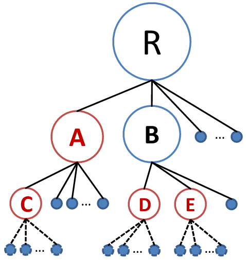 |
4.2.3 Bot-User Grouping
After pruning, a candidate connected-component may contain two or
more bot-user groups. BotGraph proceeds to decompose such
components further into individual bot-user groups. The correct
grouping is important for two reasons:
- We can extract validation features (e.g., mentioned
above and patterns of account names) more accurately from
individual bot-user groups than from a mixture of different
bot-user groups.
- Administrators may want to investigate and
take different actions on different bot-user groups based on their
behavior.
We use the random graph model to guide the process of selecting
the correct bot-user groups.
According to the random graph model, the user-user subgraph of a
bot-user group should consist of a giant connected-component plus
very small components and/or isolated vertices. So BotGraph
traverses the tree again to select tree nodes that are consistent
with such random graph property. For each node  being
traversed, there are two cases:
being
traversed, there are two cases:
- 's children contain one or more giant components whose sizes are
 , where
  is the number of users in node ;
- 's children contain only isolated vertices and/or small components with size of
 .
.
For case 1, we recursively traverse each subtree rooted by the
giant components. For case 2, we stop traversing the subtree
rooted at the . Figure 4 illustrates the
process. Here the root node  is decomposed into two giant
components
is decomposed into two giant
components  and
and  . is further decomposed into another two
giant components
. is further decomposed into another two
giant components  and
and  , while is decomposed into one
giant component
, while is decomposed into one
giant component  . The giant component disappears for any
further decomposition, indicated by the dash-lines. According to
the theory, , , , and are bot-user groups. If a node
is chosen as a bot-user group, the sub-tree rooted at the chosen
node is considered belonging to the same bot-user group. That is,
if we pick , we disregard its child as it is a subcomponent
of .
. The giant component disappears for any
further decomposition, indicated by the dash-lines. According to
the theory, , , , and are bot-user groups. If a node
is chosen as a bot-user group, the sub-tree rooted at the chosen
node is considered belonging to the same bot-user group. That is,
if we pick , we disregard its child as it is a subcomponent
of .
5 Large-scale Parallel Graph Construction
The major challenge in applying BotGraph is the construction of a large user-user graph from the Hotmail
login data - the first stage of our graph-based analysis
described in Section 3.2. Each record in
the input log data contains three fields:
UserID, IPAddress, and LoginTimestamp.
The output of the graph construction is a list of edges in the
form of UserID , UserID
 , and
Weight.
The number of users on the graph is over 500 million based on a
month-long login data (200 GB), and this number is increasing as
the Hotmail user population is growing. The number of edges of the
computed graph is on the order of hundreds of billions.
Constructing such a large graph using a single computer is
impractical. An efficient, scalable solution is required so that
we could detect attacks as early as possible in order to take
timely reactive measures.
, and
Weight.
The number of users on the graph is over 500 million based on a
month-long login data (200 GB), and this number is increasing as
the Hotmail user population is growing. The number of edges of the
computed graph is on the order of hundreds of billions.
Constructing such a large graph using a single computer is
impractical. An efficient, scalable solution is required so that
we could detect attacks as early as possible in order to take
timely reactive measures.
For data scalability, fault tolerance, and ease of programming, we
choose to implement BotGraph using Dryad/DryadLINQ, a powerful
programming environment for distributed data-parallel computing.
However, constructing a large user-user graph using
Dryad/DryadLINQ is non-trivial. This is because the resulting
graph is extremely large, therefore a straightforward
parallel implementation is inefficient in performance. In this
section, we discuss in detail our solutions. We first present both
a simple parallelism method and a selective filtering method, and
then describe several optimization strategies and their
performance impacts. We also discuss several important issues
arising in the system implementation, such as data partitioning,
data processing flow, and communication methods. Using a one-month
log as input, our current implementation can construct a graph
with tens of millions of nodes in 1.5 hours using a 240-machine
cluster. During this process, BotGraph filters out weight one
edges, and the remaining number of edges for the next-stage
processing is around 8.6 billion.
We also implemented the second stage of finding connected
components using Dryad/DryadLINQ. This stage can be solved using
the divide and conquer algorithm. In particular, one can divide
the graph edges into multiple partitions, identify the connected
subgraph components in each partition, and then merge the
incomplete subgraphs iteratively. To avoid overloading the merging
node, instead of sending all outputs to a single merging node,
each time we merge two results from two partitions. This parallel
algorithm is both efficient and scalable. Using the same
240-machine cluster in our experiments, this parallel algorithm
can analyze a graph with 8.6 billion edges in only 7 minutes --
34 times faster than the 4 hour running time by a single computer.
Given our performance bottleneck is at the first stage of graph
construction instead of graph analysis, we do not further
elaborate this step.
The first step in data-parallel applications is to partition
data. Based on the ways we partition the input data, we have different
data processing flows in implementing graph construction.
Our first approach is to partition data according to IP address,
and then to leverage the well known Map and Reduce operations to
straightforwardly convert graph construction into a data-parallel
application.
Figure 5:
Process flow of method 1
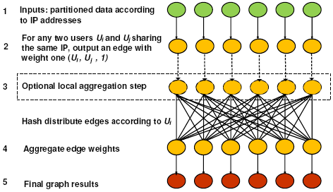 |
As illustrated in Figure 5, the input dataset is
partitioned by the user-login IP address (Step 1). During the Map
phase (Step 2 and 3), for any two users  and
and  sharing
the same IP-day pair, where the IP address is from Autonomous
System
sharing
the same IP-day pair, where the IP address is from Autonomous
System  , we output an edge with weight one
  (,
, ). Only edges pertaining to different ASes need to be
returned (Step 3). To avoid outputting the same edge multiple
times, we use a local hash table to filter duplicate edges.
(,
, ). Only edges pertaining to different ASes need to be
returned (Step 3). To avoid outputting the same edge multiple
times, we use a local hash table to filter duplicate edges.
After the Map phase, all the generated edges (from all partitions)
will serve as inputs to the Reduce phase. In particular, all edges
will be hash partitioned to a set of processing nodes for weight
aggregation using (, ) tuples as hash keys (Step 4) .
Obviously, for those user pairs that only share one IP-day in the
entire dataset, there is only one edge between them. So no
aggregation can be performed for these weight one edges. We will
show later in Figure 7 that weight one
edges are the dominate source of graph edges. Since BotGraph
focuses on only edges with weight two and above, the weight one
edges introduce unnecessary communication and computation cost to
the system. After aggregation, the outputs of the Reduce phase are
graph edges with aggregated weights.
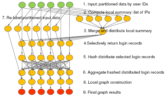
An alternative approach is to partition the inputs based on user
ID. In this way, for any two users that were located in the same
partition, we can directly compare their lists of IP-day pairs to
compute their edge weight. For two users whose records locate at
different partitions, we need to ship one user's records to
another user's partition before computing their edge weight,
resulting in huge communication costs.
We notice that for users who do not share any IP-day keys, such
communication costs can be avoided. That is, we can reduce the
communication overhead by selectively filtering data and
distributing only the related records across partitions.
Figure 6 shows the processing flow of generating
user-user graph edges with such an optimization. For each
partition  , the system computes a local summary
  to represent the union of all the IP-day keys involved in this
partition (Step 2). Each local summary is then distributed
across all nodes for selecting the relevant input records (Step
3). At each partition
to represent the union of all the IP-day keys involved in this
partition (Step 2). Each local summary is then distributed
across all nodes for selecting the relevant input records (Step
3). At each partition
 , upon receiving ,
  will return all the login records of users who shared the same
IP-day keys in . This step can be further optimized based on
the edge threshold : if a user in shares fewer than
IP-day keys with the summary , this user will not generate
edges with weight at least . Thus only the login records of
users who share at least IP-day keys with should be
selected and sent to partition (Step 4)). To ensure the
selected user records will be shipped to the right original
partition, we add an additional label to each original record to
denote their partition ID (Step 7). Finally, after partition
receives the records from partition , it joins these remote
records with its local records to generate graph edges (Step 8 and
9).
will return all the login records of users who shared the same
IP-day keys in . This step can be further optimized based on
the edge threshold : if a user in shares fewer than
IP-day keys with the summary , this user will not generate
edges with weight at least . Thus only the login records of
users who share at least IP-day keys with should be
selected and sent to partition (Step 4)). To ensure the
selected user records will be shipped to the right original
partition, we add an additional label to each original record to
denote their partition ID (Step 7). Finally, after partition
receives the records from partition , it joins these remote
records with its local records to generate graph edges (Step 8 and
9).
Other than Map and Reduce, this method requires two additional
programming interface supports: the operation to join two
heterogeneous data streams and the operation to broadcast a data
stream.
Figure 6:
Process flow of method 2.
 |
5.1.3 Comparison of the Two Methods
In general, Method 1 is simple and easy to implement, but Method 2
is more optimized for our application. The main difference between
the two data processing flows is that Method 1 generates edges of
weight one and sends them across the network in the Reduce phase,
while Method 2 directly computes edges with weight or more,
with the overhead of building a local summary and transferring the
selected records across partitions.
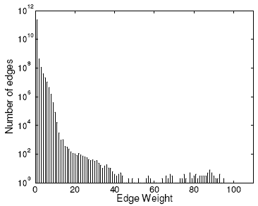
Figure 7 shows the distribution of edge
weights using one-month of user login records as input.
Here, the number of weight one edges is almost three orders of
magnitude more than the weight two edges. In our botnet detection,
we are interested in edges with a minimum weight two because
weight one edges do not show strong correlated login activities
between two users. Therefore the computation and communication
spent on generating weight one edges are not necessary. Although
in Method 1, Step 3 can perform local aggregation to reduce the
number of duplicated weight one edges, local aggregation does not
help much as the number of unique weight one edges dominates in
this case.
Figure 7:
Edge weight distribution
 |
Given our implementation is based on the existing distributed
computing models such as MapReduce and DryadLINQ, the amount of
intermediate results impacts the performance significantly because
these programming models all adopt disk read/write as cross-node
communication channels. Using disk access as communication is
robust to failures and easy to restart
jobs [6,29]. However, when the communication
cost is large such as in our case, it becomes a major bottleneck
of the overall system running time. To reduce this cost, we used a
few optimization strategies and will discuss them in the next
subsection. Completely re-designing or customizing the underlying
communication channels may improve the performance in our
application, but is beyond the scope of this paper.
Note the amount of cross-node communication also depends on the
cluster size. Method 1 results in a constant communication
overhead, i.e., the whole edge set, regardless of the number of
data partitions. But for Method 2, when the number of computers
(hence the number of data partitions) increases, both the
aggregated local summary size and the number of user-records to be
shipped increase, resulting in a larger communication overhead.
In the next subsections, we present our implementations and
evaluate the two different methods using real-data experiments.
In our implementation, we have access to a 240-machine cluster. Each
machine is configured with an AMD Dual Core 4.3G CPU and 16 GB
memory. As a pre-processing step, all the input login records were
hash partitioned evenly to the computer cluster using the DryadLINQ
built-in hash-partition function.
Given the Hotmail login data is on the order of hundreds of
Gigabytes, we spent a number of engineering efforts to reduce the
input data size and cross-node communication costs. The first two
data reduction strategies can be applied to both methods. The last
optimization is customized for Method 2 only.
1. User pre-filtering: We pre-filter users by their login AS
numbers: if a user has logged in from IP addresses across multiple
ASes in a month, we regard this user as a suspicious user
candidate. By choosing only suspicious users (using 2 ASes as the
current threshold) and their records as input, we can reduce the
number of users to consider from over 500 million (about
200-240GB) to about 70 million (about 100GB). This step completes
in about 1-2 minutes.
2. Compression: Given the potential large communication
costs, BotGraph adopts the DryadLINQ provided compression option
to reduce the intermediate result size. The use of compression
can reduce the amount of cross-node communication by 2-2.5 times.
3. Parallel data merge: In Method 2, Step 3 merges the local
IP-day summaries generated from every node and then broadcasts the
aggregated summary to the entire cluster. The old query plan
generated by DryadLINQ is shown in Figure 8 (a),
where there exists a single node that performs data aggregation
and distribution. In our experiments, this aggregating node
becomes a big bottleneck, especially for a large cluster. So we
modified DryadLINQ to generate a new query plan that supports
parallel data aggregation and distribution from every processing
node (Figure 8 (b)). We will show in
Section 5.3 that this optimization can reduce the
broadcast time by 4-5 times.
Figure 8:
(a) Default query execution plan (b) Optimized query
execution plan.
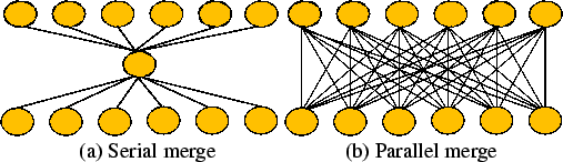 |
5.3 Performance Evaluation
In this section, we evaluate the performance of our
implementations using a one-month Hotmail user-login log collected
in Jan 2008 (referred to as the 2008-dataset). The raw input data
size is 221.5 GB, and after pre-filtering, the amount of input
data is reduced to 102.9 GB. To use all the 240 machines in the
cluster, we generated 960 partitions to serve as inputs to Method
1 (so that the computation of each partition fits into memory),
and generated 240 partitions as inputs to Method 2. With
compression and parallel data merge both enabled, our
implementation of Method 2 finishes in about 1.5 hours using all
the 240 machines, while Method 1 cannot finish within the maximum
6 hour quota allowed by the computer cluster
(Table 1). The majority of time in Method 1 is
spent on the second Reduce step to aggregate a huge volume of
intermediate results. For Method 2, the local summary selection step generated about
5.8 GB aggregated IP-day pairs to broadcast across the cluster,
resulting 1.35 TB out of the 1.7 TB total traffic.
Table 1:
Performance comparison of the two methods using the 2008-dataset.
|
|
Communication data size |
Total running time |
|
Method 1 |
12.0 TB |
 6 hours 6 hours |
|
Method 2 |
1.7 TB |
95 min |
|
In order to benchmark performance, we take a smaller dataset (about
1/5 of the full 2008-dataset) that Method 1 can finish within 6
hours. Table 2 shows the communication costs and
the total running time using the 240 machine cluster. While Method 1
potentially has a better scalability than Method 2 as discussed in
Section 5.1.3, given our practical constraints on the
cluster size, Method 2 generates a smaller amount of traffic and
outperforms Method 1 by about 5-6 times faster. The use of
compression reduces the amount of traffic by about 2-3 times, and
the total running time is about 14-25% faster.
Table 2:
Performance comparison of the two methods using a subset of the 2008-dataset.
|
|
Communication data size |
Total running time |
|
Method 1 (no comp.) |
2.71 TB |
135 min |
|
Method 1 (with comp.) |
1.02 TB |
116 min |
|
Method 2 (no comp.) |
460 GB |
28 min |
|
Method 2 (with comp.) |
181 GB |
21 min |
|
Figure 9:
Communication data size as we vary the number of input data
partitions (a) Local summary size in terms of the number of IP-day
keys. (b) Total number of selected user login records to be sent
across the network.
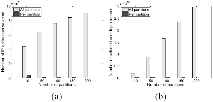 |
To evaluate the system scalability of Method 2, we vary the number
of data partitions to use different number of computers.
Figure 9 shows how the communication overheads
grow. With more partitions, the amount of data generated from
each processing node slightly decreases, but the aggregated local
summary data size increases (Figure 9 (a)). This
is because popular IP-day pairs may appear in multiple data
partitions and hence in the aggregated summary multiple times.
Similarly, the same user login records will also be shipped across
a larger number of nodes, increasing the communication costs as
the system scales (Figure 9 (b)).
Figure 10:
Running time as we vary the number of input data
partitions for Method 2. (a) Total running time of all
partitions. (b) The running of each partition. The error bars
show the max and the min running time across all partitions.
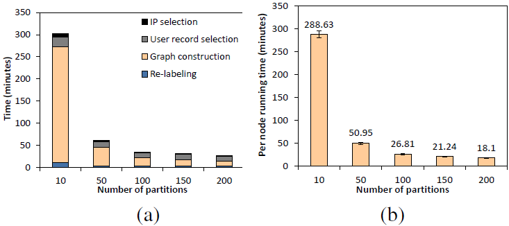 |
Even though the communication costs increase, the total running
time is still reduced with a larger cluster size.
Figure 10 (a) shows the total running time and its
breakdown across different steps. When the cluster size is small
(10 partitions), a dominant amount of time is spent on computing
the graph edges. As the system scales, this portion of time
decreases sharply. The other three steps are I/O and network
intensive. Their running time slightly decreases as we increase
the number of partitions, but the savings get diminished due to
the larger communication costs. Figure 10 (b) shows
the average running time spent on processing each partition, and
its variations are very small.
Figure 11:
(a) The processing time of user-record selection with
and without parallel data merge. (b) Minimal and maximum running
time of partitions with and without strategic data partitioning.
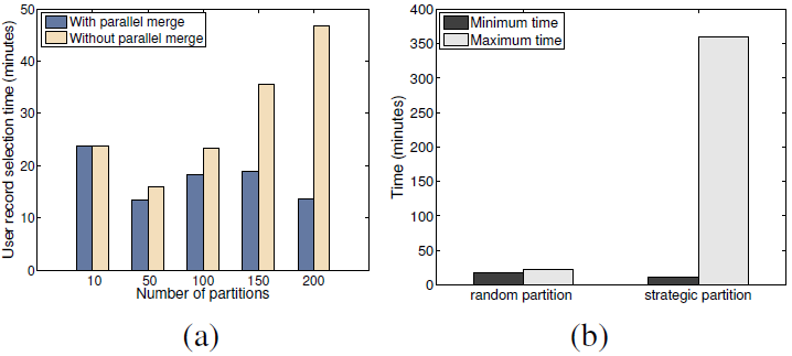 |
We now examine the benefits of adopting parallel data merge. The
purpose of parallel data merge is to remove the bottleneck node
that performs data aggregation and broadcasting. Since it is
difficult to factor out the network transfer time savings alone
(network, disk I/O, and computation are pipelined), we compare the
time spent on the user record selection step
(Figure 11 (a)). This optimization can reduce
the processing latency significantly as the cluster size increases
(75% reduction in the 200 node scenario). Without parallel data
merge, the processing time increases almost linearly, but with
this optimization, the amount of time remains roughly constant.
For Method 2, one reason for the large communication costs is that
for botnet users, their graph component is both large and dense.
Therefore, one potential optimization technique is to
strategically partition the login records. Intuitively, we can
reduce the communication costs if we pre-group users so that users
who are heavily connected are placed in one partition, and users
who are placed in different partitions have very few edges between
them. If so, Step 4 in Method 2 will return only a small number
of records to ship across different nodes. Surprisingly, we found
this strategy actually induced negative impact on the system
performance.
Figure 11 (b) shows the graph construction
time spent at a processing node with and without strategic data
partitioning. We chose the 240 input data partition scenario and
use the full dataset to illustrate the performance difference. In
the first case, we evenly distributed login records by hashing
user IDs. In the second case, we chose a large botnet user group
with 3.6M users and put all their login records evenly across 5
partitions, with the remaining data evenly distributing across the
remaining partitions. This scenario assumes the best prior
knowledge of user connections. Although in both cases, the total
amount of input data in each partition is roughly uniform, we
observe a big difference between the maximum and minimum time in
computing the edges across nodes. Without strategic partitioning,
the maximum and minimum processing time is very close. In
contrast, strategic partitioning caused a huge degree of unbalance
in workload, resulting in much longer total job running time.
6 Bot-user Detection and Validation
We use two month-long datasets as inputs to our system: a
2007-dataset collected in Jun 2007, and a 2008-dataset collected
in Jan 2008. Each dataset includes two logs: a Hotmail login log (format
described in Section 5) and a Hotmail signup
log. Each record in the signup log contains a user-ID, the remote
IP address used for signup, and the signup timestamp. For each
dataset, we run our EWMA-based anomaly detection on the signup log
and run our graph based detection on the login log. Using both
components,
BotGraph detected tens of millions of bot users and millions of botnet IPs.
Table 3 summarizes the results for both
months. We present the
detailed results and perform evaluations next.
6.1 Detection Using Signup History
Table 3:
Total Bot users and Bot IP addresses detected using both history based detection and user-user graph.
|
Month |
06/2007 |
01/2008 |
|
# of bot-users |
5.97M |
20.58M |
|
# of bot-IPs |
2.71M |
1.84M |
|
Table 4:
History based detection of bot IP addresses and bot-user
accounts.
|
Month |
06/2007 |
01/2008 |
|
# of bot IPs |
82,026 |
240,784 |
|
# of bot-user accounts |
4.83 M |
16.41 M |
|
Avg. anomaly window |
1.45 day |
1.01 day |
|
|
Table 5:
Bot IP addresses and bot-user accounts detected by
user-user graphs.
|
Month |
06/2007 |
01/2008 |
|
# of bot-groups |
13 |
40 |
|
# of bot-accounts |
2.66M |
8.68M |
|
# of unique IPs |
2.69M |
1.60M |
|
|
Table 4 shows that the EWMA algorithm detected
21.2 million bot-user accounts when applied to the two Hotmail
signup logs.
Comparing Jan 2008 with Jun 2007, both the number of bot IPs and
the signed-up bot-users increased significantly. In particular,
the total number of bot-accounts signed up in Jan 2008 is more
than three times the number in Jun 2007. Meanwhile, the anomaly
window is shortened from an average of 1.45 days to 1.01 days,
suggesting each
attack became shorter in Jan 2008.
Figure 12:
(a) Cumulative distribution of anomaly window size in terms
of number of days. (b) Cumulative distribution of the number of
accounts signed up per suspicious IP.
 |
Figure 12 (a) shows the cumulative
distribution of the anomaly window sizes associated with each bot
IP address. A majority (80% - 85%) of the detected IP addresses
have small anomaly windows, ranging from a few hours to one day,
suggesting that many botnet signup attacks happened in a burst.
Figure 12 (b) shows the cumulative
distributions of the number of accounts signed up per bot IP. As we
can see, the majority of bot IPs signed up a large number of
accounts, even though most of them have short anomaly windows.
Interestingly, the cumulative distributions derived from Jun 2007
and Jan 2008 overlap well with each other, although we observed a
much larger number of bot IPs and bot-users in Jan 2008. This
indicates that the overall bot-user signup activity patterns still
remain similar perhaps due to the reuse of bot-account signup
tools/software.
6.2 Detection by User-User Graph
We apply the graph-based bot-user detection algorithm on the
Hotmail login log to derive a tree of connected components. Each
connected component is a set of bot-user candidates. We then use
the procedures described in Section 4.2.2 to prune the
connected components of normal users. Recall that in the pruning
process, we apply a threshold on the confidence measure of each
component (computed from the ``email-per-day'' feature) to remove
normal user components.
In our experiments, the confidence measures are well separated:
most of the bot-groups have confidence measures close to 1, and a
few groups are between 0.4 and 0.6. We observe a wide margin
around confidence measure of 0.8, which we choose as our
threshold. As discussed in Section 4.2.2, this is a
conservative threshold and is in-sensitive to noises due to the
wide margin. For any group that has a confidence measure below
0.8, we regard it as a normal user group and prune it from our
tree.
Table 5 shows the final detection results
after pruning and grouping. Both the number of bot-users and the
number of bot IP addresses are on the order of millions -- a
non-trivial fraction of all the users and IP addresses observed by
Hotmail.
We find the two sets of bot-users detected in two
months hardly overlap. These accounts were stealthy ones, each sending out only a few to tens of spam
emails during the entire month.
Therefore, it is difficult to capture them by looking for aggressive sending patterns.
Due to their large population, detecting and sanitizing
these users are important both to save Hotmail resources and to
reduce the amount of spam sent to the Internet.
Comparing Jan 2008 with Jun 2007, the number of bot-users
tripled, suggesting that using Web portals as a spamming
media has become more popular.
Figure 13:
Bot-user group properties: (a) The the number of users
per group, (b) The peakness score of each group, reflecting
whether there exists a strong sharp peak for the email size
distribution.
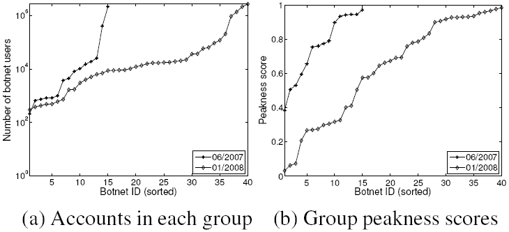 |
Now we study the properties of bot-users at a group level.
Figure 13 (a) shows that the number of users in
each group ranges from thousands to millions. Comparing Jan 2008
with Jun 2007, although the largest bot-user group remains similar
in size, the number of groups increased significantly. This
confirms our previous observation that spammers are more
frequently using Web email accounts for spam email attacks.
We next investigate the email sending patterns of the detected bot
user groups. We are interested in whether there exists a strong
peak of email sizes. We use the peakness score metric
(defined in Section 4.2.2) to quantify the degree of
email size similarity for each group. Figure 13
(b) shows the distributions of in sorted order. A majority
of groups have peakness scores higher than 0.6, meaning that over
60% of their emails have similar sizes. For the remaining groups,
we performed manual investigation and found they have multiple
peaks, resulting in lower scores. The similarity of their email
sizes is a strong evidence of correlated email sending activities.
In the next two sub-sections, we explore the quality of the total
captured 26 million bot-users. First, we examine whether they are
known bad and how many of them are our new findings. Second, we
estimate our detection false positive rates.
We evaluate our detected bot-users against a set of known spammer
users reported by other email servers in Jan 2008 5.
Denote  as the set of bot-users detected by signup history
using EWMA,
as the set of bot-users detected by signup history
using EWMA,  as the set of known spammer accounts signed up
in the month that we study, and
as the set of known spammer accounts signed up
in the month that we study, and
 as the intersection
between and . The ratio of
as the intersection
between and . The ratio of
 represents the percentage of captured bot-users that are
previously known bad. In other words,
represents the percentage of captured bot-users that are
previously known bad. In other words,
 is
our new findings. The ratio of
is
our new findings. The ratio of
 denotes the
recall of our approach. Table 6 shows
that, in Jun 2007,
85.15% of the EWMA-detected bot-user detected are already known
bad, and the detected bot-user covers a significant fraction of
bad account, i.e., recall = 67.96%.
Interestingly, Jan 2008 yields quite different results. EWMA is
still able to detect a large fraction of known bad account.
However, only 8.17% of detected bad-users were reported to be
bad. That means 91.83% of the captured spamming accounts are our
new findings.
denotes the
recall of our approach. Table 6 shows
that, in Jun 2007,
85.15% of the EWMA-detected bot-user detected are already known
bad, and the detected bot-user covers a significant fraction of
bad account, i.e., recall = 67.96%.
Interestingly, Jan 2008 yields quite different results. EWMA is
still able to detect a large fraction of known bad account.
However, only 8.17% of detected bad-users were reported to be
bad. That means 91.83% of the captured spamming accounts are our
new findings.
Table 6:
Comparing bot-users detected by signup history using EWMA
with known spammer user sets, using the ratios of
and
. See text for the definition of
and .
 |
06/2007 |
01/2008 |
 |
85.15% |
8.17% |
 |
67.96% |
52.41% |
|
|
Table 7:
Comparing bot-users detected by user-user graph with known
spammer user sets, using the ratios of
 and
and
 . See text for the definition of
  and
and
 .
.
 |
06/2007 |
01/2008 |
 |
90.95% |
45.9% |
 |
76.84% |
85.8% |
|
|
We apply a similar study to the bot-users detected by the user-user graph.
Denote as the set of known spammers users that log in from at
least 2 ASes, as the set of bot-users detected using our user-user
graph based approach, and  as the intersect between
and . Again we use the ratios of
and
to evaluate our result , as shown in
Table 7. Using our graph-based approach, the recall is higher. In total, we were able to detect
76.84% and 85.80% of known spammer users in Jun 2007 and Jan 2008, respectively. Similar to EWMA, the graph-based detection also identified a large number (54.10%) of previously unknown bot-accounts in Jan 2008. This might be because these accounts are new ones and haven't been used
aggressively to send out a massive amount of spam emails yet. So, they are not yet reported by other mail servers as of Jan 2008. The ability of detecting bot-accounts at an early stage is important to
to give us an upper hand in the anti-spam battle.
as the intersect between
and . Again we use the ratios of
and
to evaluate our result , as shown in
Table 7. Using our graph-based approach, the recall is higher. In total, we were able to detect
76.84% and 85.80% of known spammer users in Jun 2007 and Jan 2008, respectively. Similar to EWMA, the graph-based detection also identified a large number (54.10%) of previously unknown bot-accounts in Jan 2008. This might be because these accounts are new ones and haven't been used
aggressively to send out a massive amount of spam emails yet. So, they are not yet reported by other mail servers as of Jan 2008. The ability of detecting bot-accounts at an early stage is important to
to give us an upper hand in the anti-spam battle.
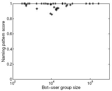
Figure 14:
Validation of login-graph detected bot-users using naming
scores.
 |
In the previous subsection, we analyzed the overlap between our
results and the set of known bad accounts. For the remaining ones,
validation is a challenging task without the ground truth. We
examine the following two account features to estimate the false
positive rates: naming patterns and signup dates.
For the identified groups, we found almost every group follows a
very clear user-name template, for example, a fixed-length
sequence of alphabets mixed with digits 6. Examples of such
names are ``w9168d4dc8c5c25f9" and ``x9550a21da4e456a2".
To quantify the similarity of account names in a group, we
introduce a naming pattern score, which is defined as the
largest fraction of users that follow a single template. Each
template is a regular expression derived by a regular expression
generation tool [27]. Since many accounts detected in Jun
2007 were known bad and hence cleaned by the system already, we
focus on bot-user groups detected in Jan 2008.
Figure 14 shows the naming score
distribution. A majority of the bot-user groups have close to 1
naming pattern scores, indicating that they were signed up by
spammers using some fixed templates. There are only a few bot-user
groups with scores lower than 0.95. We manually looked at them and
found that they are also bad users, but the user names come from
two naming templates. It is possible that our graph-based approach
mixed two groups, or the spammers purchased two groups of
bot-users and used them together. Overall, we found in total only
0.44% of the identified bot-users do not strictly follow the
naming
templates of their corresponding groups.
Our second false positive estimate is based on examining the signup
dates of the detected bot-users. Since the Web-account abuse attack
is recent and started in summer 2007, we regard all the accounts
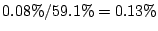
signed up before 2007 as legitimate accounts. Only 0.08% of the identified bot-users were
signed up before year 2007. To calibrate our results against the entire user population. We look at the sign up dates of all users in the input dataset.
About 59.1% of the population were signed up before 2007. Assuming the normal user signup-date distributions are the same among the overall population and our detected user set, we adjust the
false positive rate to be
The above two estimations suggest that the false positive of
BotGraph is low. We conservatively pick the higher one 0.44% as
our false positive rate estimate.
7 Discussion
In this paper, we demonstrated that BotGraph can detect tens of
millions of bot-users and millions of bots. With this
information, operators can take remedy actions and mitigate the
ongoing attacks. For bot-users, operators can block their accounts
to prevent them from further sending spam, or apply more strict
policies when they log in (e.g., request them to do additional
CAPTCHA tests). For detected bot IP addresses, one approach is to
blacklist them or rate limit their login activities, depending on
whether the corresponding IP address is a dynamically assigned
address or not. Effectively throttling botnet attacks in the
existence of dynamic IP addresses is ongoing work.
Attackers may wish to evade the BotGraph detection by developing
countermeasures.
For example, they may reduce the number of users signed up by each
bot. They may also mimic the normal user email-sending behavior by
reducing the number of emails sent per account per day (e.g.,
fewer than 3). Although mimicking normal user behavior may evade
history-based change detection or our current thresholds, these
approaches also significantly limit the attack scale by reducing
the number of bot-accounts they can obtain or the total number of
spam emails to send. Furthermore, BotGraph can still capture the
graph structures of bot-user groups from their login activity to
detect them.
A more sophisticated evasion approach may bind each bot-user to
only bots in one AS, so that our current implementation would
pre-filter them by the two AS threshold. To mitigate this attack,
BotGraph may revise the edge weight definition to look at the
number of IP prefixes instead of the number of ASes. This
potentially pushes the attacker countermeasures to be more like a
fixed IP-account binding strategy. As discussed in
Section 3.2, binding each bot-user to a
fixed bot is not desirable to the spammers. Due to the high botnet
churn rate, it would result in a low bot-user utilization rate. It
also makes attack detection easier by having a fixed group of
aggressive accounts on the same IP addresses all the time. If one
of the bot-accounts is captured, the entire group can be easily
revealed. A more generalized solution is to broaden our edge
weight definition by considering additional feature correlations.
For example, we can potentially use email sending patterns such as
the destination domain [24], email size, or email
content patterns (e.g., URL signatures [27]). As ongoing
work, we are exploring a larger set of features for more robust
attack detection.
In addition to using graphs, we may also consider other
alternatives to capture the correlated user activity. For example,
we may cluster user accounts using their login IP addresses as
feature dimensions. Given the large data volume, how to accurately
and efficiently cluster user accounts into individual bot-groups
remains a challenging research problem.
It is worth mentioning that the design and implementation of
BotGraph can be applied in different areas for constructing and
analyzing graphs. For example, in social network studies, one may
want to group users based on their buddy relationship (e.g., from
MSN or Yahoo messengers) and identify community patterns. Finally,
although our current implementations are Dryad/DryadLINQ specific,
we believe the data processing flows we propose can be potentially
generalized to other programming models.
8 Conclusion
We designed and implemented  for Web mail service
providers to defend against botnet launched Web-account abuse
attacks.
BotGraph consists of two components: a history-based
change-detection component to identify aggressive account signup
activities and a graph-based component to detect stealthy bot-user
login activities. Using two-month Hotmail logs,
successfully detected more than 26 million botnet accounts. To
process a large volume of Hotmail data, BotGraph is implemented as
a parallel Dryad/DryadLINQ application running on a large-scale
computer cluster. In this paper, we described our implementations
in detail and presented performance optimization strategies. As
general-purpose distributed computing frameworks have become
increasingly popular for processing large datasets, we believe our
experience will be useful to a wide category of applications for
constructing and analyzing large graphs.
for Web mail service
providers to defend against botnet launched Web-account abuse
attacks.
BotGraph consists of two components: a history-based
change-detection component to identify aggressive account signup
activities and a graph-based component to detect stealthy bot-user
login activities. Using two-month Hotmail logs,
successfully detected more than 26 million botnet accounts. To
process a large volume of Hotmail data, BotGraph is implemented as
a parallel Dryad/DryadLINQ application running on a large-scale
computer cluster. In this paper, we described our implementations
in detail and presented performance optimization strategies. As
general-purpose distributed computing frameworks have become
increasingly popular for processing large datasets, we believe our
experience will be useful to a wide category of applications for
constructing and analyzing large graphs.
We would like to thank Mihai Budiu, Úlfar Erlingsson, and
Dennis Fetterly for their help on DryadLINQ. We are grateful to
the Hotmail operation team for providing us with data and valuable
feedbacks. We would also like to thank Nick Feamster and anonymous
reviewers for their constructive comments.
A. EWMA based Aggressive Signup
Detection
Exponentially Weighted Moving Average (EWMA) is a well known moving
average based algorithm to detect sudden changes. EWMA is both simple and effective, and has been widely used for
anomaly detection [12].
Given a time series data, let the observation value at time  be
be
 . Let
. Let  be the predicted value at time and
  (
(
 ) be the weighting factor, EWMA predicts
as
) be the weighting factor, EWMA predicts
as
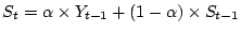 |
(1) |
We define the absolute prediction error  and the relative
prediction error
and the relative
prediction error  as:
as:
 |
(2) |
where  is introduced to avoid the divide-by-zero
problem. A large prediction error or indicates a
sudden change in the time series data and should raise an alarm.
When the number of new users signed up has dropped to the number
before the sudden change, the sudden change ends.
We define the time window between the start and the end of a sudden
change as the anomaly window.
All the accounts signed up during this anomaly window are suspicious
bot-users.
is introduced to avoid the divide-by-zero
problem. A large prediction error or indicates a
sudden change in the time series data and should raise an alarm.
When the number of new users signed up has dropped to the number
before the sudden change, the sudden change ends.
We define the time window between the start and the end of a sudden
change as the anomaly window.
All the accounts signed up during this anomaly window are suspicious
bot-users.
In our implementation, we consider the time unit of a day, and hence
is the predicted number of daily signup accounts. For any IP
address, if both
 and
and
 , we
mark day as the start of its anomaly window. From a two-year
Hotmail signup log, we derive the 99%-tile of the daily number of
account signups per IP address. To be conservative,
We set the threshold
, we
mark day as the start of its anomaly window. From a two-year
Hotmail signup log, we derive the 99%-tile of the daily number of
account signups per IP address. To be conservative,
We set the threshold
 to be twice this number to rule
out non-proxy normal IPs.
For proxies, the relative prediction error is usually a better
metric to separate them from bots. It is very rare for a proxy to
increase its signup volume by 4 times overnight. So we
conservatively set
to be twice this number to rule
out non-proxy normal IPs.
For proxies, the relative prediction error is usually a better
metric to separate them from bots. It is very rare for a proxy to
increase its signup volume by 4 times overnight. So we
conservatively set
 to 4.
to 4.


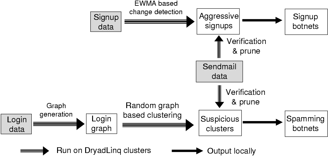
![\includegraphics[width=.45\linewidth,angle=-90]{figures/sim_graph_model_weight2.eps}](sim_graph_model_weight2.png)
![\includegraphics[width=.5\linewidth]{figures/example_email_perday.eps}](img34.png)
![\includegraphics[width=.5\linewidth]{figures/example_email_size.eps}](img35.png)
![\includegraphics[width=.5\linewidth]{figures/normal_email_perday.eps}](img36.png)
![\includegraphics[width=.5\linewidth]{figures/normal_email_size.eps}](img37.png)