Reducing Network Energy Consumption via Sleeping and Rate-Adaptation

Reducing Network Energy Consumption
via Sleeping and Rate-Adaptation

Sergiu Nedevschi1 2, Lucian Popa1 2, Gianluca Iannaccone 2, Sylvia Ratnasamy 2, David Wetherall3 4

1 University of California, Berkeley,
2 Intel Research, Berkeley,
3 Intel Research, Seattle,
4 University of Washington

Abstract

We present the design and evaluation of two forms of power management schemes that reduce the energy consumption of networks. The first is based on putting network components to sleep during idle times, reducing energy consumed in the absence of packets. The second is based on adapting the rate of network operation to the offered workload, reducing the energy consumed when actively processing packets.
For real-world traffic workloads and topologies and using power constants drawn from existing network equipment, we show that even simple schemes for sleeping or rate-adaptation can offer substantial savings. For instance, our practical algorithms stand to halve energy consumption for lightly utilized networks (10-20%). We show that these savings approach the maximum achievable by any algorithms using the same power management primitives. Moreover this energy can be saved without noticeably increasing loss and with a small and controlled increase in latency ( < 10ms). Finally, we show that both sleeping and rate adaptation are valuable depending (primarily) on the power profile of network equipment and the utilization of the network itself.

1  Introduction

In this paper, we consider power management for networks from a perspective that has recently begun to receive attention: the conservation of energy for operating and environmental reasons. Energy consumption in network exchanges is rising as higher capacity network equipment becomes more power-hungry and requires greater amounts of cooling. Combined with rising energy costs, this has made the cost of powering network exchanges a substantial and growing fraction of the total cost of ownership - up to half by some estimates[23]. Various studies now estimate the power usage of the US network infrastructure at between 5 and 24 TWh/year[25,,], or $0.5-2.4B/year at a rate of $0.10/KWh, depending on what is included. Public concern about carbon footprints is also rising, and stands to affect network equipment much as it has computers via standards such as EnergyStar. In fact, EnergyStar standard proposals for 2009 discuss slower operation of network links to conserve energy when idle. A new IEEE working group was launched in early 2007 to focus on this issue for Ethernet [15].
Fortunately, there is an opportunity for substantial reductions in the energy consumption of existing networks due to two factors. First, networks are provisioned for worst-case or busy-hour load, and this load typically exceeds their long-term utilization by a wide margin. For example, measurements reveal backbone utilizations under 30% [16] and up to hour-long idle times at access points in enterprise wireless networks [17]. Second, the energy consumption of network equipment remains substantial even when the network is idle. The implication of these factors is that most of the energy consumed in networks is wasted.
Our work is an initial exploration of how overall network energy consumption might be reduced without adversely affecting network performance. This will require two steps. First, network equipment ranging from routers to switches and NICs will need power management primitives at the hardware level. By analogy, power management in computers has evolved around hardware support for sleep and performance states. The former (e.g.,C-states in Intel processors) reduce idle consumption by powering off sub-components to different extents, while the latter (e.g.,SpeedStep, P-states in Intel processors) tradeoff performance for power via operating frequency. Second, network protocols will need to make use of the hardware primitives to best effect. Again, by analogy with computers, power management preferences control how the system switches between the available states to save energy with minimal impact on users.
Of these two steps, our focus is on the network protocols. Admittedly, these protocols build on hardware support for power management that is in its infancy for networking equipment. Yet the necessary support will readily be deployed in networks where it proves valuable, with forms such as sleeping and rapid rate selection for Ethernet [15] already under development. For comparison, computer power management compatible with the ACPI standard has gone from scarce to widely deployed over the past five to ten years and is now expanding into the server market. Thus our goal is to learn: what magnitude of energy savings a protocol using feasible hardware primitives might offer; what performance tradeoff comes with these savings; and which of the feasible kinds of hardware primitives would maximize benefits. We hope that our research can positively influence the hardware support offered by industry.
The hardware support we assume from network equipment is in the form of performance and sleep states. Performance states help to save power when routers are active, while sleep states help to save power when routers are idle. The performance states we assume dynamically change the rate of links and their associated interfaces. The sleep states we assume quickly power off network interfaces when they are idle. While link support for sleeping and rate adaptation would have seemed unlikely even in the recent past, efforts such as the recently formed IEEE 802.3az Task Force make this kinds of support a likely outcome. We develop two approaches to save energy with these primitives. The first puts network interfaces to sleep during short idle periods. To make this effective we introduce small amounts of buffering, much as 802.11 APs do for sleeping clients; this collects packets into small bursts and thereby creates gaps long enough to profitably sleep. Potential concerns are that buffering will add too much delay across the network and that bursts will exacerbate loss. Our algorithms arrange for routers and switches to sleep in a manner that ensures the buffering delay penalty is paid only once (not per link) and that routers clear bursts so as to not amplify loss noticeably. The result is a novel scheme that differs from 802.11 schemes in that all network elements are able to sleep when not utilized yet added delay is bounded. The second approach adapts the rate of individual links based on the utilization and queuing delay of the link.
We then evaluate these approaches using real-world network topologies and traffic workloads from Abilene and Intel. We find that: (1) rate-adaptation and sleeping have the potential to deliver substantial energy savings for typical networks; (2) the simple schemes we develop are able to capture most of this energy-saving potential; (3) our schemes do not noticeably degrade network performance; and (4) both sleeping and rate-adaptation are valuable depending primarily on the utilization of the network and equipment power profiles.

2  Approach

This section describes the high-level model for power consumption that motivates our rate adaptation and sleeping solutions, as well as the methodology by which we evaluate these solutions.

2.1  Power Model Overview

Active and idle power  
A network element is active when it is actively processing incoming or outgoing traffic, and idle when it is powered on but does not process traffic. Given these modes, the energy consumption for a network element is:
E = pa Ta + pi Ti
(1)
where pa, pi denote the power consumption in active and idle modes respectively and Ta, Ti the times spent in each mode.
Reducing power through sleep and performance states  
Sleep states lower power consumption by putting sub-components of the overall system to sleep when there is no work to process. Thus sleeping reduces the power consumed when idle, i.e.,it reduces the pi Ti term of Eqn. (2) by reducing the pi to some sleep-mode power draw ps where ps < pi.
Performance states reduce power consumption by lowering the rate at which work is processed. As we elaborate on in later sections, some portion of both active and idle power consumption depends on the frequency and voltage at which work is processed. Hence performance states that scale frequency and/or voltage reduce both the pa and pi power draws resulting in an overall reduction in energy consumption.
We also assume a penalty for transitioning between power states. For simplicity, we measure this penalty in time, typically milliseconds, treating it as a period in which the router can do no useful work. We use this as a simple switching model that lumps all penalties, ignoring other effects that may be associated with switches such as a transient increase in power consumption. Thus there is also a cost for switching between states.
Networks with rate adaptation and sleeping support   In a network context, the sleeping and rate adaptation decisions one router makes fundamentally impacts - and is impacted by - the decisions of its neighboring routers. Moreover, as we see later in the paper, the strategies by which each is best exploited are very different (Intuitively this is because sleep-mode savings are best exploited by maximizing idle times, which implies processing work as quickly as possible, while performance-scaling is best exploited by processing work as slowly as possible, which reduces idle times). Hence, to avoid complex interactions, we consider that the whole network, or at least well-defined components of it, run in either rate adaptation or sleep mode.
We develop the specifics of our sleeping schemes in Section  3, and our rate adaptation schemes in Section 4. Note that our solutions are deliberately constructed to apply broadly to the networking infrastructure - from end-host NICs, to switches, and IP routers, etc. - so that they may be applied wherever they prove to be the most valuable. They are not tied to IP-layer protocols.

2.2  Methodology

The overall energy savings we can expect will depend on the extent to which our power-management algorithms can successful exploit opportunities to sleep or rate adapt as well as the power profile of network equipment (i.e.,, relative magnitudes of pa, pi and ps). To clearly separate the effect of each, we evaluate sleep solutions in terms of the fraction of time for which network elements can sleep and rate-adaptation solutions in terms of the reduction in the average rate at which the network operates 1. In this way we assess each solution with the appropriate baseline. We then evaluate how these metrics translate into overall network energy savings for different equipment power profiles and hence compare the relative merits of sleeping and rate-adaptation (Section 5). For both sleep and rate-adaptation, we calibrate the savings achieved by our practical solutions by comparing to the maximum savings achievable by optimal, but not necessarily practical, solutions.
In network environments where packet arrival rates can be highly non-uniform, allowing network elements to transition between operating rates or sleep/active modes with corresponding transition times can introduce additional packet delay, or even loss, that would have not otherwise occurred. Our goal is to explore solutions that usefully navigate the tradeoff between potential energy savings and performance. In terms of performance, we measure the average and 98th percentile of the end-to-end packet delay and loss.
In the absence of network equipment with hardware support for power management, we base our evaluations on packet-level simulation with real-world network topologies and traffic workloads. The key factors on which power savings then depend, beyond the details of the solutions themselves, are the technology constants of the sleep and performance states and the characteristics of the network. In particular, the utilization of links determines the relative magnitudes of Tactive and Tidle as well as the opportunities for profitably exploiting sleep and performance states. We give simple models for technology constants in the following sections. To capture the effect of the network on power savings, we drive our simulation with two realistic network topologies and traffic workloads (Abilene and Intel) that are summarized below. We use ns2 as our packet-level simulator.
Abilene   We use Abilene as a test case because of the ready availability of detailed topology and traffic information. The information from [27] provides us with the link connectivity, weights (to compute routes), latencies and capacities for Abilene's router-level topology. We use measured Abilene traffic matrices (TMs) available in the community [29] to generate realistic workloads over this topology. Unless otherwise stated, we use as our default a traffic matrix whose link utilization levels reflect the average link utilization over the entire day - this corresponds to a 5% link utilization on average with bottleneck links experiencing about 15% utilization.
We linearly scale TMs to study performance with increasing utilization up to a maximum average network utilization of 31% as beyond this some links reach very high utilizations. Finally, while the TMs specify the 5-minute average rate observed for each ingress-egress pair, we still require a packet-level traffic generation model that creates this rate. In keeping with previous studies [18,31] we generate traffic as a mix of Pareto flows, and for some results we use constant bit-rate (CBR) traffic. As per standard practice, we set router queue sizes equal to the bandwidth-delay product in the network; we use the bandwidth of the bottleneck link, and a delay of 100ms.
Intel   As an additional real-world dataset, we collected topology and traffic information for the global Intel enterprise network. This network connects Intel sites worldwide, from small remote offices to large multi-building sites with thousands of users. It comprises approximately 300 routers and over 600 links with capacities ranging from 1.5Mbps to 1Gbps.
To simulate realistic traffic, we collected unsampled Netflow records [6] from the core routers. The records, exported by each router every minute, contain per flow information that allows us to recreate the traffic sourced by ingress nodes.

3  Putting Network Elements to Sleep

In this section we discuss power management algorithms that exploit sleep states to reduce power consumption during idle times.

3.1  Model and Assumptions

Background   A well established technique, as used by microprocessors and mobiles, is to reduce idle power by putting hardware sub-components to sleep. For example, modern Intel processors such as the Core Duo [1] have a succession of sleep states (called C-states) that offer increasingly reduced power at the cost of increasingly high latencies to enter and exit these states. We assume similar sleep states made available for network equipment. For the purpose of this study we ignore the options afforded by multiple sleep states and assume as an initial simplification that we have a single sleep state.
Model  
We model a network sleep state as characterized by three features or parameters. The first is the power draw in sleep mode ps which we assume to be a small fraction of the idle mode power draw pi.
The second characterizing parameter of a sleep state is the time δ it takes to transition in and out of sleep states. Higher values of δ raise the bar on when the network element can profitably enter sleep mode and hence δ critically affects potential savings. While network interface cards can make physical-layer transitions in as low as 10ms, transition times that involve restoring state at higher layers (memory, operating system) are likely to be higher [13]. We thus evaluate our solutions over a wide range values of transition times.
Finally, network equipment must support a mechanism for invoking and exiting sleep states. The option that makes the fewest assumptions about the sophistication of hardware support is timer-driven sleeping, in which the network element enters and exits sleep at well-defined times. Prior to entering sleep the network element specifies the time in the future at which it will exit sleep and all packets that arrive at a sleeping interface are lost. The second possibility, described in [12], is for routers to wake up automatically on sensing incoming traffic on their input ports. To achieve this "wake-on-arrival" (WoA), the circuitry that senses packets on a line is left powered on even in sleep mode. While support for WoA is not common in either computers or interfaces today, this is a form of hardware support that might prove desirable for future network equipment and is currently under discussion in the IEEE 802.3az Task Force [13]. Note that even with wake-on-arrival, bits arriving during the transition period δ are effectively lost. To handle this, the authors in [6] propose the use of "dummy" packets to rouse a sleeping neighbor. A node A that wishes to wake B first sends B a dummy packet, and then waits for time δ before transmitting the actual data traffic. The solutions we develop in this paper apply seamlessly to either timer-driven or WoA-based hardware.
Measuring savings and performance   In this section, we measure savings in terms of the percentage of time network elements spend asleep and performance in terms of the average and 98th percentile of the end-to-end packet delay and loss. We assume that individual line cards in a network element can be independently put to sleep. This allows for more opportunities to sleep than if one were to require that a router sleep in its entirety (as the latter is only possible when there is no incoming traffic at any of the incoming interfaces). Correspondingly our energy savings are with respect to interface cards which typically represent a major portion of the overall consumption of a network device. That said, one could in addition put the route processor and switch fabric to sleep at times when all line cards are asleep.

3.2  Approaches and Potential savings

For interfaces that support wake-on-arrival, one approach to exploiting sleep states is that of opportunistic sleeping in which link interfaces sleep when idle - i.e.,a router is awakened by an incoming (dummy) packet and, after forwarding it on, returns to sleep if no subsequent packet arrives for some time. While very simple, such an approach can result in frequent transitions which limits savings for higher transition times and/or higher link speeds. For example, with a 10Gbps link, even under low utilization (5%) and packet sizes of 1KB, the average packet inter-arrival time is very small - 15ms. Thus while opportunistic sleeping might be effective in LANs [11,22] with high idle times, for fast links this technique is only effective for very low transition times δ (we quantify this shortly). In addition, opportunistic sleep is only possible with the more sophisticated hardware support of wake-on-arrival.
To create greater opportunities for sleep, we consider a novel approach that allows us to explicitly control the tradeoff between network performance and energy savings. Our approach is to shape traffic into small bursts at the edges of the network - edge devices then transmit packets in bunches and routers within the network wake up to process a burst of packets, and then sleep until the next burst arrives. The intent is to provide sufficient bunching to create opportunities for sleep if the load is low, yet not add excessive delay. This is a radical approach in the sense that much other work seeks to avoid bursts rather than create them (e.g., token buckets for QOS, congestion avoidance, buffering at routers). As our measurements of loss and delay show, our schemes avoid the pitfalls associated with bursts because we introduce only a bounded and small amount of burstiness and a router never enters sleep until it has cleared all bursts it has built up. More precisely, we introduce a buffer interval "B" that controls the tradeoff between savings and performance. An ingress router buffers incoming traffic for up to B ms and, once every B ms, forwards buffered traffic in a burst.
figures/motivate-peregress.png
Figure 1: Packets within a burst are organized by destination.
To ensure that bursts created at the ingress are retained as they traverse through the network, an ingress router arranges packets within the burst such that all packets destined for the same egress router are contiguous within the burst (see figure 1).
The above "buffer-and-burst" approach (B&B) creates alternating periods of contiguous activity and sleep leading to fewer transitions and amortizing the transition penalty δ over multiple packets. This improvement comes at the cost of an added end-to-end delay of up to B ms. Note that because only ingress routers buffer traffic, the additional delay due to buffering is only incurred once along the entire ingress-to-egress path. As importantly, this approach - unlike opportunistic sleep - can be used by interfaces that support only timer-driven sleep. A router R1 that receives a burst from upstream router R2 at time t1 knows that the next start-of-burst will arrive at time t1+B and can hence sleep between bursts.
figures/sleepy_combined.png
Figure 2: Examples of burst synchronization.
The question then is how significant are the savings this approach enables for reasonable additional delay? We note that the best possible savings would occur if a router received the incoming bursts from all ingress routers close in time such that it processes all incoming bursts and returns to sleep thus incurring exactly one sleep/wake transition per B ms. This might appear possible by having ingress routers coordinate the times at which they transmit bursts such that bursts from different ingresses arrive close in time at intermediate routers. For example, consider the scenario in Figure 2(a) where ingress routers R0 and R1 are scheduled to transmit traffic at times 2 and 1 respectively. If instead R1 were to schedule its burst for time 7 instead, then bursts from R0 and R2 would align in time at R2 thus reducing the number of distinct burst times - and sleep-to-wake transitions - at downstream routers R3 and R4.
Unfortunately, the example in Figure 2(b) suggests this is unachievable for general topologies. Here, Si and Sj represent the arrival times of incoming bursts to nodes R3 and R1 respectively and we see that the topology makes it impossible to find times Si and Sj that could simultaneously align the bursts downstream from R2 and R4.
We thus use a brute-force strategy to evaluate the maximum achievable coordination. For a given topology and traffic workload, we consider the start-of-burst time for traffic from each ingress I to egress J (denoted Sij) and perform an exhaustive search of all Sij to find a set of start times that minimizes the number of transitions across all the interfaces in the network. We call this scheme optB&B. Clearly, such an algorithm is not practical and we use it merely as an optimistic bound on what might be achievable were nodes to coordinate in shaping traffic under a buffer-and-burst approach.
We compare the sleep time achieved by optB&B to the upper bound on sleep as given by 1 - m, where m is the network utilization. This upper bound is not achievable by any algorithm since (unlike optB&B) it does not take into account the overhead δ due to sleep/wake transitions. Nonetheless it serves to capture the loss in savings due to δ and the inability to achieve perfect coordination.
Any traffic shaping incurs some additional complexity and hence a valid question is whether we need any traffic shaping, or whether opportunistic sleeping that does not require shaping is enough? We therefore also compare optB&B to opportunistic sleeping based on wake-on-arrival (WoA). For this naive WoA, we assume optimistically that an interface knows the precise arrival time of the subsequent packet and returns to sleep only for inter-packet arrival periods greater than δ. Because the performance of opportunistic WoA depends greatly on the inter-arrival times of packets we evaluate WoA for two types of traffic: constant bit rate (CBR) and Pareto.
figures/sleep_opt_woa.png
Figure 3: Time asleep using optB&B and opportunistic sleeping and compared to the upper bound (1-m).
For each of the above bounds, Figure 3 plots the percentage of time asleep under increasing utilization in Abilene. We use a buffer period of B=10ms and assume a (conservative) transition time δ of 1ms. Comparing the savings from optB&B to the utilization bound, we see that a traffic shaping approach based on buffer-and-burst can achieve much of the potential for exploiting sleep. As expected, even at very low utilization, WoA with CBR traffic can rarely sleep; perhaps more surprising is that even with bursty traffic WoA performs relatively poorly. These results suggest that - even assuming hardware WoA - traffic shaping offers a significant improvement over opportunistic sleep.

3.3  A Practical Algorithm

We consider a very simple buffer-and-burst scheme, called practB&B, in which each ingress router sends its bursts destined for the various egresses one after the other in a single "train of bursts". At routers close to the ingress this appears as a single burst which then disperses as it traverses through the network.
practB&B bounds the number of bursts (and correspondingly the number of transitions) seen by any router R in an interval of B ms to at most IR, the total number of ingress routers that send traffic through R. In practice, our results show that the number of bursts seen by R in time Bms is significantly smaller than this bound.
practB&B is simple - it requires no inter-router coordination as the time at which bursts are transmitted is decided independently by each ingress router. For networks supporting wake-on-arrival the implementation is trivial - the only additional feature is the implementation of buffer-and-burst at the ingress nodes. For networks that employ timer-driven sleeping, packet bursts would need to include a marker denoting the end of burst and notifying the router of when it should expect the next burst on that interface.

3.4  Evaluation

We evaluate the savings vs. performance tradeoff achieved by practB&B algorithm and the impact of equipment and network parameters on the same.
Savings vs. performance using practB&B   We compare the sleep time achieved by practB&B to that achievable by optB&B. In terms of performance, we compare the end-to-end packet delay and loss in a network using practB&B to that of a network that never sleeps (as today) as this shows the overall performance penalty due to our sleep protocols.
figures/sleep_opt_pract_pareto_cbr.png
Figure 4: Time asleep using CBR and Pareto traffic.
Figure 4 plots the sleep time with increasing utilization on the Abilene network using a buffering interval B=10ms. We plot the percentage sleep time under both CBR and Pareto traffic workloads. We see that even a scheme as simple as practB&B can create and exploit significant opportunities for sleep and approaches the savings achieved by the significantly more complex optB&B. As with opportunistic sleeping, we see that practB&B's savings with CBR traffic are lower than for the more bursty Pareto workloads, but that this reduction is significantly smaller in the case of practB&B than with opportunistic sleeping (recall Figure 3). That Pareto traffic improves savings is to be expected as burstier traffic only enhances our bunching strategy.
Figures 5(a) and (b) plot the corresponding average and 98th percentile of the end-to-end delay. As expected, we see that the additional delay in both cases is proportional to the buffering interval B. Note that this is the end-to-end delay, reinforcing that the buffering delay B is incurred once for the entire end-to-end path.
We see that for higher B, the delay grows slightly faster with utilization (e.g.,compare the absolute increase in delay for B=5ms to 25ms) because this situation is more prone to larger bursts overlapping at intermediate routers. However this effect is relatively small even in a situation combining larger B (25ms) and larger utilizations (20-30%) and is negligible for smaller B and/or more typical utilizations.
We see that both average and maximum delays increase abruptly beyond network utilizations exceeding 25%. This occurs when certain links approach full utilization and queuing delays increase (recall that the utilization on the horizontal axis is the average network-wide utilization). However this increase occurs even in the default network scenario and is thus not caused by practB&B's traffic shaping.
Finally, our measurements revealed that practB&B introduced no additional packet loss (relative to the default network scenario) until we approach utilizations that come close to saturating some links. For example, in a network scenario losses greater than 0.1% occur at 41% utilization without any buffering, they occur at 38% utilization with B=10ms, and at 36% utilization with B=25. As networks do not typically operate with links close to saturation point, we do not expect this additional loss to be a problem in practice.
In summary, the above results suggest that practB&B can yield significant savings with a very small (and controllable) impact on network delay and loss. For example, at a utilization of 10%, a buffering time of just B=5ms allows the network to spend over 60% of its time in sleep mode for under 5ms added delay.
figures/sleep_avg_delay.png figures/sleep_max_delay.png
Figure 5: The impact on delay of practB&B.
Impact of hardware characteristics   We now evaluate how the transition time δ affects the performance of practB&B  Figure 6(a) plots the sleep time achieved by practB&B for a range of transition times and compares this to the ideal case of having instantaneous transitions. As expected, the ability to sleep degrades drastically with increasing δ. This observation holds across various buffer intervals B as illustrated in Figure 6(b) that plots the sleep time achieved at typical utilization ( » 5%) for increasing transition times and different values of B.
figures/sleeptime_ts.png figures/sleep_graph3.png
Figure 6: The impact of hardware constants on sleep time.
These findings reinforce our intuition that hardware support featuring low-power sleep states and quick transitions (preferably < 1ms) between these states are essential to effectively save energy.
Impact of network topology   We now evaluate practB&B for the Intel enterprise network. The routing structure of the Intel network is strictly hierarchical with a relatively small number of nodes that connect to the wide-area. Because of this we find a wide variation in link utilization - far more than on the Abilene network. Over 77% of links have utilizations below 1% while a small number of links ( 2.5%) can see significantly higher utilizations of between 20-75%. Correspondingly, the opportunity for sleep also varies greatly across links. This is shown in Figure 7 - each point in the scatter-plot corresponds to a single link and we look at sleep times for two transition times: 0.1ms and 1ms. We see that the dominant trends in sleep time vs. utilization remains and that higher δ yields lower savings.
figures/new_intel/intel_sleepy.png
Figure 7: Time asleep per link

4  Rate-Adaptation in Networks

This section explores the use of performance states to reduce network energy consumption.

4.1  Model and Assumptions

Background   In general, operating a device at a lower frequency can enable dramatic reductions in energy consumption for two reasons. First, simply operating more slowly offers some fairly substantial savings. For example, Ethernet links dissipate between 2-4W when operating between 100Mbps-1Gbps compared to 10-20W between 10Gbps[10]. Second, operating at a lower frequency also allows the use of dynamic voltage scaling (DVS) that reduces the operating voltage. This allows power to scale cubically, and hence energy consumption quadratically, with operating frequency[32]. DVS and frequency scaling are already common in microprocessors for these reasons.
We assume the application of these techniques to network links and associated equipment (i.e., linecards, transceivers). While the use of DVS has been demonstrated in prototype linecards [21], it is not currently supported in commercial equipment and hence we investigate savings under two different scenarios: (1) equipment that supports only frequency scaling and (2) equipment that supports both frequency and voltage scaling.
Model   We assume individual links can switch performance states independently and with independent rates for transmission and reception on interfaces. Hence the savings we obtain apply directly to the consumption at the links and interface cards of a network element, although in practice one could also scale the rate of operation of the switch fabric and/or route processor.
We assume that each network interface supports N performance states corresponding to link rates r1, ¼, rn (with ri < ri+1 and rn = rmax, the default maximum link rate), and we investigate the effect that the granularity and distribution (linear vs. exponential) of these rates has on the potential energy savings.
The final defining characteristic of performance states is the transition time, denoted δ, during which packet transmission is stalled as the link transitions between successive rates. We explore performance for a range of transition times (δ) from 0.1 to 10 milliseconds.
Measuring savings and performance  
As in the case of sleep we're interested in solutions that reduce the rate at which links operate without significantly affecting performance.
In this section, we use the percentage reduction in average link rate as an indicative measure of energy savings and relate this to overall energy savings in Section 5 where we take into account the power profile of equipment (including whether it supports DVS or not). In terms of performance, we again measure the average and 98th percentile of the end-to-end packet delay and packet loss.

4.2  An optimal strategy

Our initial interest is to understand the extent to which performance states can help if used to best effect. For a DVS processor, it has been shown that the most energy-efficient way to execute C cycles within a given time interval T is to maintain a constant clock speed of C/T [20]. In the context of a network link, this translates into sending packets at a constant rate equal to the average arrival rate. However under non-uniform traffic this can result in arbitrary delays and hence we instead look for an optimal schedule of rates (i.e.,the set of rates at which the link should operate at different points in time) that minimize energy while respecting a specified constraint on the additional delay incurred at the link.
More precisely, given a packet arrival curve AC, we look for a service curve SC that minimizes energy consumption, while respecting a given upper bound d on the per-packet queuing delay. The delay parameter d thus serves to tradeoff savings for increased delay. Figure 8(a) shows an example arrival curve and the associated latest-departure curve (AC+d), which is simply the arrival curve shifted in time by the delay bound d. To meet the delay constraint, the service curve SC must lie within the area between the arrival and latest-departure curves.
figures/figsc2.png
Figure 8: An illustration of delay-constrained service curves and the service curve minimizing energy.
In the context of wireless links, [19] proves that if the energy can be expressed as a convex, monotonically increasing function of the transmission rate, then the minimal energy service curve is the shortest Euclidean distance in the arrival space (bytes × time) between the arrival and shifted arrival curves.
In the scenario where we assume DVS support, the energy consumption is a convex, monotonically increasing function of link rate and thus this result applies to our context as well. Where only frequency scaling is supported, any service curve between the arrival and shifted-arrival curves would achieve the same energy savings and therefore the service curve with the shortest Euclidean distance would be optimal in this case too. In summary, for both frequency-scaling and DVS, the shortest distance service curve would achieve the highest possible energy savings.
Fig. 8 illustrates an example of such a minimal energy service curve. Intuitively, this is the set of lowest constant rates obeying the delay constraint. Note that this per-link optimal strategy is not suited to practical implementation since it assumes perfect knowledge of the future arrival curve, link rates of infinite granularity and ignores switching overheads. Nonetheless, it is useful as an estimate of the potential savings by which to calibrate practical protocols.
We will evaluate the savings achieved by applying the above per-link solution at all links in the network and call this approach link_optRA. One issue in doing so is that the service curves at the different links are inter-dependent - i.e., the service curve for a link l depends in turn on the service curves at other links (since the latter in turn determine the arrival curve at l). We address this by applying the per-link optimal algorithm iteratively across all links until the service and arrival curves at the different links converge.

4.3  A practical algorithm

Building on the insight offered by the per-link optimal algorithm, we develop a simple approach, called practRA (practical rate adaptation), that seeks to navigate the tradeoff between savings and delay constraints. A practical approach differs from the optimum in that (i) it does not have knowledge of future packet arrivals, (ii) it can only choose among a fixed set of available rates r1, ¼, rn, and (iii) at every rate switch, it incurs a penalty δ, during which it cannot send packets.
While knowledge of the future arrival rate is unavailable, we can use the history of packet arrivals to predict the future arrival rate. We denote this predicted arrival rate as [^r]f and estimate it with an exponentially weighted moving average (EWMA) of the measured history of past arrivals. Similarly, we can use the current link buffer size q and rate ri to estimate the potential queuing delay so as to avoid violating the delay constraint.
With these substitutes, we define a technique inspired by the per-link optimal algorithm. In practRA, packets are serviced at a constant rate until we intersect one of the two bounding curves presented earlier (Figure 8): the arrival curve (AC), and the latest-departure curve (AC+d). Thus, we avoid increasing the operating rate ri unless not doing so would violate the delay constraint. This leads to the following condition for rate increases:
A link operating at rate ri with current queue size q increases its rate to ri+1 iff ([q/(ri)] > d OR [(δ[^r]f + q)/(ri+1)] > d - δ)
The first term checks whether the delay bound d would be violated were we to maintain the current link rate. The second constraint ensures that the service curve does not get too close to the delay-constrained curve which would prevent us from attempting a rate increase in the future without violating the delay bound. That is, we need to allow enough time for a link that increases its rate to subsequently process packets that arrived during the transition time (estimated by δ·[^r]f) and its already-accumulated queue. Note that we cannot use delay constraints d smaller than the transition time δ.
Similarly, the condition under which we allow a rate decrease is as follows:
A link operating at rate ri with current queue size q decreases its rate to ri-1 iff    q = 0 AND [^r]f < ri-1
First, we only attempt to switch to a lower rate when the queue at the link is empty (q=0). Intuitively, this corresponds to an intersection between the arrival curve and the service curve. However, we don't always switch to a lower rate ri-1 when a queue empties as doing so would prevent the algorithm from operating in a (desired) steady state mode with zero queuing delay. Instead, the desirable steady state is one where ri > rf > ri+1 and we want to avoid oscillating between rates (which would lead to larger average delay). For example, a link that sees a constant arrival rate of 3.5Mbps might oscillate between 3 and 4Mbps (incurring queuing delays at 3Mbps), instead of remaining at 4Mbps (with low average queuing delay). We thus use the additional condition: [^r]f < ri-1  to steer our algorithm toward the desired steady state and ensure that switching to a lower rate does not immediately lead to larger queues.
In addition to the above conditions, we further discourage oscillations by enforcing a minimum time K δ between consecutive switches. Intuitively, this is because rate switching should not occur on timescales smaller than the transition time δ. In our experiments, we found K=4 to be a reasonable value for this parameter.
Note that unlike the link_optRA algorithm, the above decision process does not guarantee that the delay constraints will be met since it is based on estimated rather than true arrival rates. Similarly, practRA cannot guarantee that the rates used by the links match those used by the link-optimal algorithm. In section 5, after discussing how power scales with rate, we use simulation to compare our approximate algorithm to the optimal under realistic network conditions. We leave it to future work to analytically bound the inaccuracy due to our approximations.
Finally, we observe that the above rate-adaptation is simple in that it requires no coordination across different nodes, and is amenable to implementation in high-speed equipment. This is because the above decision making need not be performed on a per-packet basis.

4.4  Evaluation

We evaluate the savings vs. performance tradeoff achieved by our practical rate-adaptation algorithm and the impact of equipment and network parameters on the same. We first evaluate the percentage reduction in average link rate achieved by practRA for the Abilene network. For comparison, we consider the rate reduction due to link_optRA and the upper bound on rate reduction as determined by the average link utilization. In this case, since we found the reduction from link_optRA was virtually indistinguishable from the utilization bound, we only show the latter here for clarity. (We report on the energy savings due to link_optRA in the following section.) To measure performance, we measure the end-to-end packet delay and loss in a network using practRA to that in a network with no rate adaptation.
Impact of hardware characteristics  
The main constants affecting the performance of practRA are (1) the granularity and distribution of available rates, and (2) δ, the time to transition between successive rates. We investigate the reduction in rate for three different distributions of rates r1,..., rn: (i) 10 rates uniformly distributed between 1Gbps to 10Gbps, (ii) 4 rates uniformly distributed between 1Gbps to 10Gbps and (iii) 4 exponentially distributed rates (10Gbps, 1Gbps, 100Mbps, 10Mbps). We consider the latter case since physical layer technologies for these rates already exist making these likely candidates for early rate-adaptation technologies.
Figure 9 plots the average rate reduction under increasing utilizations, with a per-link delay constraint d = δ + 2ms, and a transition time δ = 1ms. We see that for 10 uniformly distributed rates, practRA operates links at a rate that approaches the average link utilization. With 4 uniformly distributed rates this reduction drops, but not significantly. However, for exponentially distributed rates, the algorithm performs poorly, indicating that support for uniformly distributed rates is essential.
figures_slides/rate_utilization_time.png
Figure 9: Average rate of operation. The average is weighted by the time spent at a particular rate.
figures_slides/rate_avg_delay.png figures_slides/rate_top_delay.png
Figure 10: Average and 98th percentile delay achieved by practRA for various available rates
Figure 10 plots the corresponding average and 98th percentile of the end-to-end delay. We see that, for all the scenarios, the increase in average delay due to practRA is very small: ~ 5ms in the worst case, and less than 2ms for the scenario using 4 uniform rates. The increase in maximum delay is also reasonable: at most 78ms with practRA, relative to 69ms with no adaptation.
Perhaps surprisingly, the lowest additional delay occurs in the case of 4 uniformly distributed rates. We found this occurs because there are fewer rate transitions, with corresponding transition delays, in this case. . Finally, we found that practRA introduced no additional packet loss for the range of utilizations considered.
Next, we look at the impact of transition times δ. Figures 11 (a) and (b) plot the average rate reduction and 98th percentile of delay under increasing δ for different network utilizations. For each test, we set the delay constraint as d = δ+ 2ms, and we assume 10 uniform rates. As would be expected, we see that larger δ lead to reduced savings and higher delay. On the whole we see that, in this scenario, both savings and performance remain attractive for transition times as high as ~ 2ms.
figures_slides/ts_vs_savings_lin_time.png figures/rate_nsdi/top_delay_ts_u.png
Figure 11: Impact of Switch Time (δ) for practRA
In summary, these results suggest that rate adaptation as implemented by practRA has the potential to offers significant energy savings with little impact on packet loss or delay. In all our tests, we found practRA to have minimal effects on the average delay and loss and hence, from here on, we measure the performance impact only in terms of the 98th percentile in packet delay.
Impact of network topology   We now evaluate practRA applied to the Intel enterprise network. Figure 12 plots the rate reduction across links - each point in the scatter-plot corresponds to a single link, and we look at rate reduction for two rate distribution policies: 10 uniformly distributed rates and 4 exponentially distributed rates. Since these are per-link results, we see significant variations in rate reduction for the same utilization, due to specifics of traffic across various links. We also notice that the dominant trend in reduction remains similar to that seen in the Abilene network (Figure 9).
figures/new_intel/intel_rate.png
Figure 12: Rate reduction per link

5  Overall Energy Savings

In the previous sections we evaluated power-management solutions based on their ability to increase sleep times (Section  3), or operate at reduced rates (Section  4). In this section, we translate these to overall energy savings and hence compare the relative merits of rate adaptation vs. sleeping. For this, we develop an analytical model of power consumption under different operating modes. Our model derives from measurements of existing networking equipment[13,4,24]. At the same time, we construct the model to be sufficiently general that we may study the potential impact of future, more energy-efficient, hardware.

5.1  Power Model

Recall from section 2 that the total energy consumption of a network element operating in the absence of any power-saving modes can be approximated as: E = pa Ta + pi Ti.
We start by considering the power consumption when actively processing packets (pa). Typically, a portion of this power draw is static in the sense that it does not depend on the operating frequency (e.g., refresh power in memory blocks, leakage currents and so forth) while the dominant portion of power draw does scale with operating frequency. Correspondingly, we set:

pa(r) = C + f(r)
(2)
Intuitively, C can be viewed as that portion of power draw that cannot be eliminated through rate adaptation while f(r) reflects the rate-dependent portion of energy consumption. To reflect the relative proportions of C and f(r) we set C to be relatively small - between 0.1 and 0.3 of the maximum active power pa(rn). To study the effect of just frequency scaling alone we set f(r)=O(r) and set f(r)=O(r3) to evaluate dynamic voltage scaling (DVS). In evaluating DVS, we need to consider an additional constraint - namely that, in practice, there is a minimum rate threshold below which scaling the link rate offers no further reduction in voltage. We thus define a maximum scaling factor λ and limit our choice of available operating rates to lie between [rn/λ, rn], for scenarios that assume voltage scaling. While current transistor technology allows scaling up to factors as high as 5 [32], current processors typically use λ ~ 2 and hence we investigate both values as potential rate scaling limits.
Empirical measurements further reveal that the idle mode power draw, pi, varies with operating frequency in a manner similar to the active-mode power draw but with lower absolute value[13]. Correspondingly, we model the idle-mode power draw as:
pi(r) = C + βf(r)
(3)
Intuitively, the parameter β represents the relative magnitudes of routine work incurred even in the absence of packets to the work incurred when actively processing packets. While measurements from existing equipment suggest values of β as high as 0.8 for network interface cards [13] and router linecards [4], we would like to capture the potential for future energy-efficient equipment and hence consider a wide range of β between [0.1, 0.9].
Energy savings from rate adaptation   With the above definitions of pa and pi, we can now evaluate the overall energy savings due to rate adaptation. The total energy consumption is now given by:

Σ
rk 
pa(rk)Ta(rk) + pi(rk)Ti(rk)
(4)
Our evaluation in Section 4 yields the values of Ta(rk) and Ti(rk) for different rk and test scenarios, while Eqns. 2 and  3 allow us to model pa(rk) and pi(rk) for different C, β and f(r). We first evaluate the energy savings using rate adaptation under frequency scaling (f(r)=O(r)) and DVS (f(r)=O(r3)). For these tests, we set C and β to middle-of-the-range values of 0.2 and 0.5 respectively; we examine the effect of varying C and β in the next section.
figures/new_savings/savings_util_lin_policy.png figures/new_savings/savings_util_dvs_policy.png figures/new_savings/sleep_gamma_util.png
Figure 13: Total Energy Saving with Sleeping and Rate Adaptation

Figure 13(a) plots the energy savings for our practical (practRA) and optimal (link_optRA) rate adaptation algorithms assuming only frequency scaling. We see that, in this case, the relative energy savings for the different algorithms as well as the impact of the different rate distributions is similar to our previous results (Fig. 9) that measured savings in terms of the average reduction in link rates. Overall, we see that significant savings are possible even in the case of frequency scaling alone.
Figure 13(b) repeats the above test assuming voltage scaling for two different values of λ, the maximum rate scaling factor allowed by DVS. In this case, we see that the use of DVS significantly changes the savings curve - the more aggressive voltage scaling allows for larger savings that can be maintained over a wide range of utilizations. Moreover, we see that once again the savings from our practical algorithm (practRA) approach those from the optimal algorithm. Finally, as expected, increasing the range of supported rates (λ) results in additional energy savings.
Energy savings from sleeping   To model the energy savings with sleeping, we need to pin down the relative magnitudes of the sleep mode power draw (ps) relative to that when idle (pi). We do so by introducing a parameter γ and set:
ps = γpi(rn)
(5)
where 0.0 £ γ £ 1.0. While the value of γ will depend on the hardware characteristics of the network element in question, empirical data suggest that sleep mode power is typically a very small fraction of the idle-mode power consumption: ~ 0.02 for network interfaces [13], 0.001 for RFM radios [11], 0.3 for PC cards [11] and less than 0.1 for DRAM memory [7]. In our evaluation we consider values of γ between 0 and 0.3.
With this, the energy consumption of an element that spends time Ts in sleep is given by:
E = pa(rn) Ta + pi(rn)(Ti - Ts) + ps Ts.
(6)
Our evaluation from Section 3 estimated Ts for different scenarios. Figure 13(c) plots the corresponding overall energy savings for different values of γ for our practB&B algorithm. We assume a transition time δ = 1ms, and a buffering interval B=10ms. Again, our results confirm that sleeping offers good overall energy savings and that, as expected, energy savings are directly proportional to γ.

5.2  Comparison: Sleep vs. Rate Adaptation

We now compare the savings from sleeping vs. rate adaptation by varying the two defining axes of our power model: C, the percentage of power that doesn't scale with frequency, and β that determines the relative magnitudes of idle to active power draws. We consider two end-of-the-range values for each: C=0.1 and C=0.3 and β = 0.1 and β = 0.8. Combining the two gives us four test cases that span the spectrum of hardware power profiles:
We evaluate energy savings for each of the above scenarios for the case where the hardware supports DVS and when the hardware only supports frequency scaling.
With DVS: f(r)=O(r3)   Figures 14 plots the overall energy savings for practRA and practB&B for the different test scenarios. These tests assume 10 uniformly distributed rates and a sleep power ps = 0.1 pi(rn). In each case, for both sleep and rate-adaptation, we consider hardware parameters that reflect the best and worst case savings for the algorithm in question. For practRA, these parameters are λ (the range for voltage scaling) and δ (the transition time). For the best-case results these are λ = 5 and δ = 0.1ms; for the worst case: λ = 2, δ = 1ms. The parameter for practB&B is the transition time δ which we set as δ = 0.1ms (best case) and δ = 1ms (worst case).
The conclusion we draw from Figure 14 is that, in each scenario there is a "boundary" utilization below which sleeping offers greater savings, and above which rate adaptation is preferable. Comparing across graphs, we see that the boundary utilization depends primarily on the values of C and β, and only secondarily on the transition time and other hardware parameters of the algorithm. For example, the boundary utilization for C=0.1 and β = 0.1 varies between approximately 5-11% while at C=0.3,β = 0.8 this boundary utilization lies between 4% and 27%. We also evaluated savings under different traffic characteristics (CBR, Pareto) and found that the burstiness of traffic has a more secondary effect on the boundary utilization.
figures/new_comparisons/c01_b01_comp_dvs.png figures/new_comparisons/c01_b08_comp_dvs.png figures/new_comparisons/c03_b01_comp_dvs.png figures/new_comparisons/c03_b08_comp_dvs.png
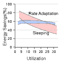
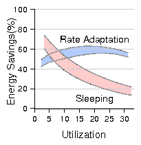
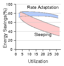
Figure 14: Comparison of energy savings between sleep and rate adaptation. Support for dynamic voltage scaling.
For further insight on what determines the boundary utilization, we consider the scenario of a single idealized link. The sleep-mode energy consumption of such an idealized link can be viewed as:
Esleep = pa(rmax) mT + ps(1-m)T
(7)
Similarly, the idealized link with rate adaptation is one that runs with an average rate of mrmax for an energy consumption of:
Erate = pa(mrmax)T
(8)
Figure 15 represents the boundary utilization for this idealized link as a function of C. In this idealized scenario, the dominant parameter is C because the link is never idle and therefore β has only a small, indirect effect on ps. The gray zone in the figure represents the spread in boundary utilization obtained by varying β between 0.1 and 0.9.
figures/new_comparisons/c_util_threshold.png
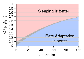
Figure 15: Sleeping vs. rate-adaptation
With frequency scaling alone: f(r)=O(r)   
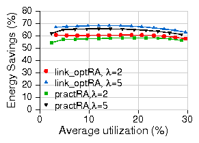
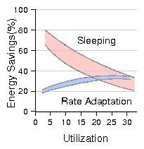
Figures 16 plots the overall energy savings for practRA and practB&B for the different test scenarios in the more pessimistic scenario where voltage scaling is not supported. Due to lack of space, we only plot the comparison for the first two test scenarios where C=0.1; at C=0.3, the savings show a similar scaling trend but with significantly poorer performance for rate-adaptation and hence add little additional information.
The primary observation is that the savings from rate adaptation are significantly lower than in the previous case with DVS and, in this case, sleeping outperforms rate adaptation more frequently. We also see that - unlike the DVS case - network utilization impacts energy savings in a similar manner for both sleeping and rate-adaptation (i.e., the overall "slope" of the savings-vs-utilization curves is similar with both sleeping and rate-adaptation while they were dramatically different with DVS - see Fig. 14).
Once again, we obtain insight on this by studying the the highly simplified case of a single idealized link. For this idealized scenario with f(r)=O(r), we find that the boundary condition that determines whether to use sleep or rate adaptation is in fact independent of network utilization. Instead, one can show that sleep is superior to rate-adaptation if the following inequality holds:
c > γβ

1 - γ( 1 - β)
(9)
Otherwise, rate adaptation is superior.
In practice, network utilization does play a role (as our results clearly indicate) because the various practical constraints due to delay bounds and transition times prevent our algorithms from fully exploiting all opportunities to sleep or change rates.
In summary, we find that both sleeping and rate-adaptation are useful, with the tradeoff between them depending primarily on the power profile of hardware capabilities and network utilization. Results such as those presented here can guide operators in deciding how to best run their networks. For example, an operator might choose to run the network with rate adaptation during the day and sleeping at night based on where the boundary utilization intersects diurnal behavior, or identify components of the network with consistently low (or high) utilization to be run with sleeping (or rate-adaptation).
figures/new_comparisons/c01_b01_comp_lin.png figures/new_comparisons/c01_b08_comp_lin.png
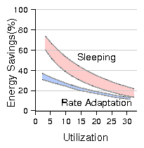
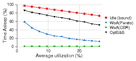
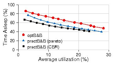
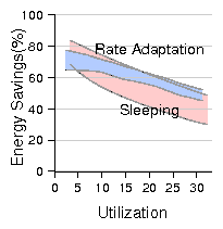
Figure 16: Energy savings of sleep vs. rate adaptation, β = 0.1, frequency scaling alone.

6  Related Work

There is a large body of work on power management in contexts complementary to ours. This includes power provisioning and load balancing in data centers[5,8], and OS techniques to extend battery lifetimes in mobiles[9,30].
Perhaps the first to draw attention to the problem of saving overall energy in the network was an early position paper by Gupta et al. [12]. They use data from the US Department of Commerce to detail the growth in network energy consumption and argue the case for energy-saving network protocols, including the possibility of wake-on-arrival in wired routers. In follow-on work they evaluate the application of opportunistic sleeping in a campus LAN environment [22,11].
Other recent work looks at powering-down redundant access points (APs) in enterprise wireless networks [17]. The authors propose that a central server collect AP connectivity and utilization information to determine which APs can be safely powered down. This approach is less applicable to wired networks that exhibit much less redundancy.
Sleeping has also been explored in the context of 802.11 to save client power, e.g., see [2]. The 802.11 standard itself includes two schemes (Power-Save Poll and Automatic Power Save Delivery) by which access points may buffer packets so that clients may sleep for short intervals. In some sense, our proposal for bunching traffic to improve sleep opportunities can be viewed as extending this idea deep into the network.
Finally, the IEEE Energy Efficient Ethernet Task Force has recently started to explore both sleeping and rate adaptation for energy savings. Some initial studies consider individual links and are based on synthetic traffic and infinite buffers [3].
In the domain of sensor networks, there have been numerous efforts to design energy efficient protocols. Approaches investigated include putting nodes to sleep using TDMA-like techniques to coordinate transmission and idle times (e.g., FPS [14]), and distributed algorithms for sleeping (e.g.,S-MAC [28]). This context differs from ours in many ways.

7  Conclusion

We have argued that power management states that slow down links and put components to sleep stand to save much of the present energy expenditure of networks. At a high-level, this is apparent from the facts that while network energy consumption is growing networks continue to operate at low average utilizations. We present the design and evaluation of simple power management algorithms that exploit these states for energy conservation and show that - with the right hardware support - there is the potential for saving much energy with a small and bounded impact on performance, e.g., a few milliseconds of delay. We hope these preliminary results will encourage the development of hardware support for power saving as well as algorithms that use them more effectively to realize greater savings.

Aknowledgments

We thank Robert Hays, Bob Grow, Bruce Nordman, Rabin Patra and Ioan Bejenaru for their suggestions. We also thank the anonymous reviewers and our shepherd Jon Crowcroft for their useful feedback.
.90

References

[1]
Power and Thermal Management in the Intel Core Duo Processor. In Intel Technology Review, Volume 10, Issue 2, Section 4. 2006.
[2]
Y. Agarwal, R. Chandra, et al. Wireless wakeups revisited: energy management for voip over wi-fi smartphones. In ACM MobiSys. 2007.
[3]
C. Gunaratne and K. Christensen and B. Nordman and S. Suen. Reducing the energy consumption of Ethernet with Adaptive Link Rate (ALR). In IEEE Transactions on Computers. April, 2008.
[4]
J. Chabarek, J. Sommers, et al. Power awareness in network design and routing. In INFOCOM 2008. 2008.
[5]
J. S. Chase, D. C. Anderson, et al. Managing energy and server resources in hosting centers. In ACM SOSP. 2001.
[6]
Cisco Systems. NetFlow services and applications. White Paper, 2000.
[7]
X. Fan, C. S. Ellis, et al. Memory Controller Policies for DRAM Power Management. In International Symposium on Low Power Electronics and Design. 2003.
[8]
X. Fan, W.-D. Weber, et al. Power provisioning for a warehouse-sized computer. In ACM ISCA. 2007.
[9]
J. Flinn and M. Satyanarayanan. Energy-aware adaptation for mobile applications. In ACM SOSP. 1999.
[10]
C. Gunaratne, K. Christensen, et al. Managing Energy Consumption Costs in Desktop PCs and LAN Switches with Proxying, Split TCP Connections, and Scaling of Link Speed. In International Journal of Network Management. October 2005.
[11]
M. Gupta, S. Grover, et al. A feasibility study for power management in lan switches. In ICNP. 2004.
[12]
M. Gupta and S. Singh. Greening of the internet. In ACM SIGCOMM, Karlsruhe, Germany. August 2003.
[13]
R. Hays. Active/Idle Toggling with Low-Power Idle, http://www.ieee802.org/3/az/public/jan08/hays_01_0108 .pdf. In IEEE 802.3az Task Force Group Meeting. 2008.
[14]
B. Hohlt, L. Doherty, et al. Flexible power scheduling for sensor networks. In IEEE and ACM Third International Symposium on Information Processing in Sensor Networks (IPSN). April 2004.
[15]
IEEE 802.3 Energy Efficient Ethernet Study Group. http://grouper.ieee.org/groups/802/3/eee_study/.
[16]
Ipmon Sprint. The Applied Research Group. http://ipmon.sprint.com/.
[17]
A. Jardosh, G. Iannaccone, et al. Towards an Energy-Star WLAN Infrastructure. In HOTMOBILE. 2007.
[18]
S. Kandula, D. Katabi, et al. Walking the tightrope: Responsive yet stable traffic engineering. In ACM SIGCOMM 2005.
[19]
M. Lin and Y. Ganjali. Power-efficient rate scheduling in wireless links using computational geometric algorithms. In IWCMC. 2006.
[20]
J. Lorch. Operating systems techniques for reducing processor energy consumption. In Ph.D. Thesis, University of California, Berkeley. 1994.
[21]
M. Mandviwalla and N.-F. Tzeng. Energy-efficient scheme for multiprocessor-based router linecards. In IEEE SAINT. 2006.
[22]
Maruti Gupta and Suresh Singh. Dynamic Ethernet Link Shutdown for Energy Conservation on Ethernet Links. In IEEE ICC. 2007.
[23]
E. Miranda and L. McGarry. Power/thermal impact of networking computing. In Cisco System Research Symposium, August, 2006.
[24]
S. Nedevschi. Reducing network energy consumption via sleeping and rate-adaptation, http://www.ieee802.org/3/az/public/jan08/nedevschi_01 _0108.pdf. In IEEE 802.3az Task Force Group Meeting. 2008.
[25]
B. Nordman. Energy Efficient Ethernet, Outstanding Questions. 2007.
[26]
K. W. Roth, F. Goldstein, et al. Energy Consumption by Office and Telecommunications Equipment in Commercial Buildings - Volume I: Energy Consumption Baseline. Tech. Rep. 72895-00, Arthur D. Little, Inc, Jan. 2002.
[27]
The Abilene Observatory. http://abilene.internet2.edu/. observatory.
[28]
W. Ye, J. Heidemann, et al. An energy-efficient mac protocol for wireless sensor networks. In ACM INFOCOM. 2002.
[29]
Yin Zhang's AbileneTM,http://www.cs.utexas.edu/ yzhang. /research/AbileneTM.
[30]
W. Yuan and K. Nahrstedt. Energy-efficient soft real-time cpu scheduling for mobile multimedia systems. In ACM SOSP. 2003.
[31]
M. Yuksel, B. Sikdar, et al. Workload generation for ns simulations of wide area networks and the internet. In Communication Networks and Distributed Systems Modeling and Simulation Conference. 2000.
[32]
B. Zhai, D. Blaauw, et al. Theoretical and practical limits of dynamic voltage scaling. In DAC. 2004.

Notes:

1 In reality the energy savings using rate-adaptation will depend on the distribution of operating rates over time and the corresponding power consumption at each rate. For simplicity, we initially use the average rate of operation as an indirect measure of savings in Section 4 and then consider the complete distribution of operating rates in Section 5 when we compute energy savings.