|
NSDI '06 Paper
[NSDI '06 Technical Program]
Open Versus Closed: A Cautionary Tale
Open Versus Closed: A Cautionary Tale
Bianca Schroeder
Carnegie Mellon University
Pittsburgh, PA 15213
bianca@cs.cmu.edu
Adam Wierman
Carnegie Mellon University
Pittsburgh, PA 15213
acw@cs.cmu.edu
Mor Harchol-Balter
Carnegie Mellon University
Pittsburgh, PA 15213
harchol@cs.cmu.edu
Abstract
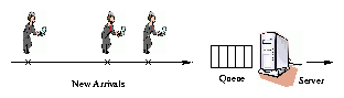
Workload generators may be classified as based on a closed system
model, where new job arrivals are only triggered by job
completions (followed by think time), or an open system model,
where new jobs arrive independently of job completions. In
general, system designers pay little attention to whether a
workload generator is closed or open.
Using a combination of implementation and simulation experiments,
we illustrate that there is a vast difference in behavior between
open and closed models in real-world settings. We synthesize these
differences into eight simple guiding principles, which serve
three purposes. First, the principles specify how scheduling
policies are impacted by closed and open models, and explain the
differences in user level performance. Second, the principles
motivate the use of partly open system models, whose behavior we
show to lie between that of closed and open models. Finally, the
principles provide guidelines to system designers for determining
which system model is most appropriate for a given workload.
1 Introduction
Every systems researcher is well aware of the importance of
setting up one's experiment so that the system being modeled is
"accurately represented." Representing a system accurately
involves many things, including accurately representing the
bottleneck resource behavior, the scheduling of requests at that
bottleneck, and workload parameters such as the distribution of
service request demands, popularity distributions, locality
distributions, and correlations between requests. However, one
factor that researchers typically pay little attention to is
whether the job arrivals obey a closed or an open system model. In
a closed system model, new job arrivals are only triggered
by job completions (followed by think time), as in
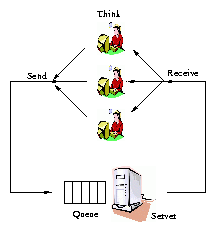
Figure 1(a). By contrast in an open system
model, new jobs arrive independently of job completions, as in
Figure 1(b).
|
(a) Closed system
|
| |
|
(c) Partly-open system
|
| |
Figure 1: Illustrations of the closed, open, and
partly-open system models.
Table 1 surveys the system models in a variety
of web related workload generators used by systems researchers
today. The table is by no means complete; however it illustrates
the wide range of workload generators and benchmarks available.
Most of these generators/benchmarks assume a closed system model,
although a reasonable fraction assume an open one. For many of
these workload generators, it was quite difficult to figure out
which system model was being assumed - the builders often do not
seem to view this as an important factor worth mentioning in the
documentation. Thus the "choice" of a system model (closed
versus open) is often not really a researcher's choice, but rather
is dictated by the availability of the workload generator. Even
when a user makes a conscious choice to use a closed model, it is
not always clear how to parameterize the closed system (e.g. how
to set the think time and the multiprogramming level - MPL) and
what effect these parameters will have.
In this paper, we show that closed and open system models yield
significantly different results, even when both models are run
with the same load and service demands. Not only is the measured
response time different under the two system models, but the two
systems respond fundamentally differently to varying parameters and to
resource allocation (scheduling) policies.
We obtain our results primarily via real-world implementations.
Although the very simplest models of open and closed systems can be
compared analytically, analysis alone is insufficient to capture the
effect of many of the complexities of modern computer systems,
especially size based scheduling and realistic job size
distributions. Real-world implementations are also needed to capture
the magnitude of the differences between closed and open systems in
practice. The case studies we consider are described in Section
4. These include web servers receiving static HTTP
requests in both a LAN and a WAN setting; the back-end database in e-commerce applications; and an
auctioning web site. In performing
these case studies, we needed to develop a flexible suite of workload
generators, simulators, and trace analysis tools that can be used
under closed, open, and other system models. The details of this
suite are also provided in Section 4.
Our simulation and implementation experiments lead us to identify
eight principles, summarizing the observed differences
between open and closed system models, many of which are not
obvious. These principles may be categorized by their area of
impact.
The first set of principles (see Section
5.1) describe the difference in mean
response time under open and closed system models and how
various parameters affect these differences. We find, for
example, that for a fixed load, the mean response time for an open
system model can exceed that for a closed system model by an order
of magnitude or more. Even under a high MPL, the
closed system model still behaves "closed" with respect to mean
response time, and there is still a significant difference between
mean response times in closed and open systems even for an MPL of
1000. With respect to service demands (job sizes), while their
variability has a huge impact on response times in open systems,
it has much less of an effect in closed models. The impact of
these principles is that a system designer needs to beware of
taking results that were discovered under one system model (e.g. closed model) and
applying them to a second system model (e.g. open model).
The second set of principles (see Section 5.2) deal
with the impact of scheduling on improving system performance.
Scheduling is a common mechanism for improving mean response time
without purchasing additional resources. While Processor-Sharing
scheduling (PS) and First-Come-First-Served (FCFS) are most commonly
used in computer systems, many system designs give preference to
short jobs (requests with small service demands), applying policies
like Non-Preemptive-Shortest-Job-First (SJF) or
Preemptive-Shortest-Job-First (PSJF) to disk scheduling
[51] and web server scheduling
[19,33,15].
When system designers seek to evaluate a new scheduling policy, they
often try it out using a workload generator and simulation test-bed.
Our work will show that, again, one must be very careful that one is
correctly modeling the application as closed or open, since the
impact of scheduling turns out to be very different under open and
closed models. For example, our principles show that favoring short
jobs is highly effective in improving mean response time in open
systems, while this is far less true under a closed system model. We
find that closed system models only benefit from scheduling under a
narrow range of parameters, when load is moderate and the MPL is very
high. The message for system designers is that understanding
whether the workload is better modeled with an open or closed system
is essential in determining the effectiveness of scheduling.
|
| Type of benchmark | Name | System model | |
| Model-based web workload generator | Surge [10], WaspClient [31], Geist [22], WebStone [47], | Closed |
| WebBench [49], MS Web Capacity Analysis Tool [27] | |
| SPECWeb96 [43], WAGON [23] | Open |
| Playback mechanisms for HTTP request | MS Web Application Stress Tool [28], Webjamma [2], | |
| streams | Hammerhead [39], Deluge [38], Siege [17] | Closed |
| httperf [30], Sclient [9] | Open |
| Proxy server benchmarks | Wisconsin Proxy Benchmark [5], Web Polygraph [35], Inktomi Climate Lab [18] | Closed |
| Database benchmark for e-commerce workloads | TPC-W [46] | Closed |
| Auction web site benchmark | RUBiS[7] | Closed |
| Online bulletin board benchmark | RUBBoS[7] | Closed |
| Database benchmark for online transaction processing (OLTP) | TPC-C [45] | Closed |
| Model-based packet level web traffic | IPB (Internet Protocol Benchmark) [24], GenSyn [20] | Closed |
| generators | WebTraf [16], trafgen [14] | |
| NS traffic generator [52] | Open |
| Mail server benchmark | SPECmail2001 [42] | Open |
| Java Client/Server benchmark | SPECJ2EE [41] | Open |
| Web authentication and authorization | AuthMark [29] | Closed |
| Network file servers | NetBench [48] | Closed |
| SFS97_R1 (3.0) [40] | Open |
| Streaming media service | MediSyn [44] | Open | |
Table 1: A summary table of the system models
underlying standard web related workload generators.
The third set of principles (see Section 6)
deal with partly-open systems. We observe that while
workload generators and benchmarks typically assume either an open
system model or a closed system model, neither of these is
entirely realistic. Many applications are best represented using
an "in-between" system model, which we call the partly-open
model. Our principles specify those parameter settings for which
the partly-open model behaves more like a closed model or more
like an open model with respect to response time. We also find
that, counter to intuition, parameters like think time have almost
no impact on the performance of a partly-open model. The
principles describing the behavior of the partly-open system model
are important because real-world applications often fit best into
partly-open models, and the performance of these models is not
well understood. In particular, the effect of system parameters
and scheduling on performance in the partly open system - points
which our principles address - are not known. Our results
motivate the importance of designing versatile workload
generators that are able to support open, closed, and partly open
system models. We create such versatile workload generators for
several common systems, including web servers and database
systems, and use these throughout our studies.
The third set of principles also provides system designers with
guidelines for how to choose a system model when they are
forced to pick a workload generator that is either purely closed
or purely open, as are almost all workload generators (see
Section 7). We consider ten different workloads and
use our principles to determine for each workload which system
model is most appropriate for that workload: closed, open, or
partly-open. To the best of our knowledge, no such guide exists
for systems researchers.
2 Closed, open, and partly-open systems
In this section, we define how requests are generated under
closed, open, and partly-open system models.
Figure 1(a) depicts a closed system
configuration. In a closed system model, it is assumed that there
is some fixed number of users, who use the system forever. This
number of users is typically called the multiprogramming
level (MPL) and denoted by N. Each of these N users repeats
these 2 steps, indefinitely: (a) submit a job, (b) receive the
response and then "think" for some amount of time. In a closed
system, a new request is only triggered by the completion of
a previous request. At all times there are some number of users,
Nthink, who are thinking, and some number of users
Nsystem, who are either running or queued to run in the
system, where Nthink + Nsystem = N. The response
time, T, in a closed system is defined to be the time from when
a request is submitted until it is received. In the case where the
system is a single server (e.g. a web server), the server
load, denoted by r, is defined as the fraction of time that
the server is busy, and is the product of the mean throughput X
and the mean service demand (processing requirement) E[S].
Figure 1(b) depicts an open system
configuration. In an open system model there is a stream of
arriving users with average arrival rate l. Each user is
assumed to submit one job to the system, wait to receive the
response, and then leave. The number of users queued or running
at the system at any time may range from zero to infinity. The
differentiating feature of an open system is that a request
completion does not trigger a new request: a new request is only
triggered by a new user arrival. As before, response
time, T, is defined as the time from when a request is
submitted until it is completed. The server load is defined
as the fraction of time that the server is busy. Here load,
r, is the product of the mean arrival rate of requests,
l, and the mean service demand E[S].
Neither the open system model nor the closed system model is
entirely realistic. Consider for example a web site. On the one
hand, a user is apt to make more than one request to a web site,
and the user will typically wait for the output of the first
request before making the next. In these ways a closed system
model makes sense. On the other hand, the number of users at the
site varies over time; there is no sense of a fixed number of
users N. The point is that users visit to the web site, behave
as if they are in a closed system for a short while, and then
leave the system.
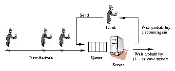
Motivated by the example of a web site, we study a more realistic
alternative to the open and closed system configurations: the
partly-open system shown in Figure 1(c). Under the
partly-open model, users arrive according to some outside arrival
process as in an open system. However, every time a user completes
a request at the system, with probability p the user stays and
makes a followup request (possibly after some think time), and
with probability 1-p the user simply leaves the system. Thus the
expected number of requests that a user makes to the system in a
visit is Geometrically distributed with mean 1/(1-p). We refer
to the collection of requests a user makes during a visit to the
system as a session and we define the length of a
session to be the number of requests in the session/visit. The
server load is the fraction of time that the server is busy
equaling the product of the average outside arrival rate
l, the mean number of requests per visit E[R], and the
mean service demand E[S]. For a given load, when p is small,
the partly-open model is more similar to an open model. For large
p, the partly-open model resembles a closed model.
3 Comparison methodology
In this section we discuss the relevant parameters and metrics for
both the open and the closed system models and discuss how we set
parameters in order to compare open and closed system models.
Throughout the paper we choose the service demand distribution to
be the same for the open and the closed system. In the case
studies the service demand distribution is either taken from a
trace or determined by the benchmark used in the experiments. In
the model-based simulation experiments later in the paper, we use
hyperexponential service demands, in order to capture the highly
variable service distributions in web applications. Throughout, we
measure the variability in the service demand distribution using
the square coefficient of variation, C2. The think time in the
closed system, Z, follows an exponential distribution, and the
arrival process in the open system is either a Poisson arrival
process with average rate l, or is provided by
traces.1
The results for all simulations and experiments are presented in
terms of mean response times and the system load r. While we
do not explicitly report numbers for another important metric,
mean throughput, the interested reader can directly infer those
numbers by interpreting load as a simple scaling of throughput. In
an open system, the mean throughput is simply equal to l = r/E[S], which is the same as throughput in a closed system.
In order to fairly compare the open and closed systems, we
will hold the system load r for the two systems equal, and
study the effect
of open versus closed system models on mean response time.
The load in the open system is specified by l, since r = lE[S]. Fixing the load of a closed system is more
complex, since the load is affected by many parameters including
the MPL, the think time, the service demand variability, and the
scheduling policy. The fact that system load is influenced by many
more system parameters in a closed system than in an open system
is a surprising difference between the two systems.
Throughout, we will achieve a desired system load by adjusting the
think time of the closed system (see Figure 7(a)), while
holding all other parameters fixed.
The scheduling policies we study in this work span the range of
behaviors of policies that are used in computer systems today.
- FCFS
- (First-Come-First-Served) Jobs are processed in the
same order as they arrive.
- PS
- (Processor-Sharing) The server is shared evenly among
all jobs in the system.
- PESJF
- (Preemptive-Expected-Shortest-Job-First) The job with
the smallest expected duration (size) is given preemptive priority.
- SRPT
- (Shortest-Remaining-Processing-Time-First): At
every moment the request with the smallest remaining processing
requirement is given priority.
- PELJF
- (Preemptive-Expected-Longest-Job-First) The job
with the longest expected size is given preemptive priority. PELJF
is an example of a policy that performs badly and is included to
understand the full range of possible response times.
4 Real-world case studies
In this section, we compare the behavior of four different
applications under closed, open, and partly open system models. The
applications include (a) a web server delivering static content in a
LAN environment, (b) the database back-end at an e-commerce web site,
(c) the application server at an auctioning web site, and (d) a web
server delivering static content in a WAN environment. These applications vary in many respects, including the bottleneck
resource, the workload properties (e.g. job size variability),
network effects, and the types of scheduling policies considered.
We study applications (a), (b), and (d) through full
implementation in a real test-bed, while our
study of application (c) relies on trace-based simulation.
As part of the case studies, we develop a set of workload generators,
simulators, and trace analysis tools that facilitate experimentation
with all three system models: open, closed, and partly-open. For
implementation-based case studies we extend the existing workload
generator (which is based on only one system model) to enable all
three system models. For the case studies based on trace-driven
simulation, we implement a versatile simulator that models open,
closed, and partly-open systems and takes traces as input. We also
develop tools for analyzing web traces (in Common Logfile Format or
Squid log format) to extract the data needed to parameterize workload
generators and simulators.
Sections 4.1 - 4.4 provide the details of the case studies. The main results are shown
in Figures 2 and 4. For each case study we
first explain the tools developed for experimenting in open, closed,
and partly-open models. We then then describe the relevant scheduling
policies and their implementation, and finally discuss the results.
The discussions at the end of the case studies are meant only
to highlight the key points; we will discuss the differences between
open, closed, and partly-open systems and the impact of these
differences in much more detail in Sections 5 and
6.
|
 Closed System |
|
| |
|
|
Open System |
|
| |
|
|
Partly-open System
(a) Static web - LAN |
|
| |
|
Closed System |
|
| |
|
Open System |
|
| |
|
Partly-open System
(b) E-commerce site |
|
| |
|
Closed System |
|
| |
|
Open System |
|
| |
|
Partly-open System
(c) Auctioning site
|
|
| |
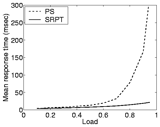
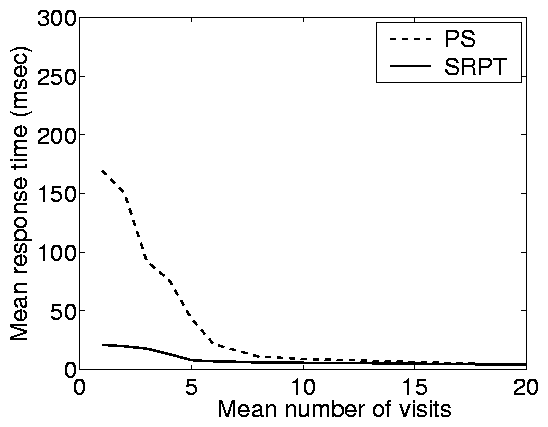
Figure 2: Results for real-world case studies. Each row
shows the results for a real-world workload and each column shows
the results for one of the system models. In all experiments with
the closed system model the MPL is 50. The partly-open system is
run at fixed load 0.9.
4.1 Static web content
Our first case study is an Apache web server running on Linux and
serving static content, i.e. requests of the form "Get me a
file," in a LAN environment. Our experimental setup involves six
machines connected by a 10/100 Ethernet switch. Each machine has
an Intel Pentium III 700 MHz processor and 256 MB RAM, and runs
Linux. One of the machines is designated as the server and runs
Apache. The others generate web requests based on a web trace.
Workload generation: In this case
study we generate static web workloads based on a trace. Below we
first describe our workload generator which generates web requests
following an open, closed, or partly-open model. We then describe
the tool for analyzing web traces that produces input files needed
by the workload generator. Finally we briefly describe the actual
trace that we are using in our work.
Our workload generator is built on top of the
Sclient[9] workload generator. The Sclient
workload generator uses a simple open system model, whereby a new
request for file y is made exactly every x msec.
Sclient is designed as a single process that manages all connections
using the select system call. After each call to select,
Sclient checks whether the current x msec interval has passed
and if so initiates a new request.
We generalize Sclient in several ways.
For the open system, we change Sclient to make requests based on
arrival times and filenames specified in an input file. The
entries in the input file are of the form < ti, fi > , where
ti is a time and fi is a file name.
For the closed system, the input file only specifies the names of the files
to be requested. To implement closed system arrivals in Sclient,
we have Sclient maintain a list with the times when the next
requests are to be made. Entries to the list are generated during
runtime as follows:
Whenever a request completes, an exponentially distributed think time Z is
added to the current time tcurr and the result Z+tcurr is inserted into the list of
arrival times.
In the case of the partly-open system, each entry in the input file
now defines a session, rather than an individual request. An entry
in the input file takes the form < ti, fi1, ¼, fin >
where ti specifies the arrival time of the session and
< fi1, ¼, fin > is the list of files to be requested
during the session. As before, a list with arrival times is maintained
according to which requests are made. The list is initialized with
the session arrival times ti from the input file.
To generate the arrivals within a session, we use the same method
as described for the closed system above: after request fij-1 completes
we arrange the arrival of request fij by adding an entry
containing the arrival time Z+tcurr to the list, where tcurr
is the current time and Z is an exponentially distributed think time.
All the input files for the workload generator are created based
on a web trace. We modify the Webalizer tool [12] to
parse a web trace and then extract the information needed to
create the input files for the open, closed, and partly-open
system experiments. In the case of the open system, we simply
output the arrival times together with the names of the requested
files. In the case of the closed system, we only extract the
sequence of file names. Creating the input file for the
partly-open system is slightly more involved since it requires
identifying the sessions in a trace. A common approach for
identifying sessions (and the one taken by Webalizer) is to group
all successive requests by the same client
(i.e. same IP address) into one session, unless the time between
two requests exceeds some timeout threshold in which case a new
session is started. In our experiments, we use the timeout
parameter to specify the desired average session length.
The trace we use consists of one day from the 1998 World Soccer
Cup, obtained from the Internet Traffic Archive [21].
Virtually all requests in this trace are static.
|
| Number | Mean | Variability | Min | Max |
| of Req. | size | (C2) | size | size |
| 4.5·106 | 5KB | 96 | 41 bytes | 2MB | |
Scheduling: Standard scheduling of
static requests in a web server is best modeled by processor
sharing (PS). However, recent research suggests favoring requests
for small files can improve mean response times at web servers
[19]. In this section we
therefore consider both PS and SRPT policies.
We have modified the Linux kernel and the Apache Web server to
implement SRPT scheduling at the server. For static HTTP
requests, the network (access link out of the server) is typically
the bottleneck resource. Thus, our solution schedules the
bandwidth on this access link by controlling the order in which
the server's socket buffers are drained. Traditionally, the
socket buffers are drained in Round-Robin fashion (similar to PS);
we instead give priority to sockets corresponding to connections
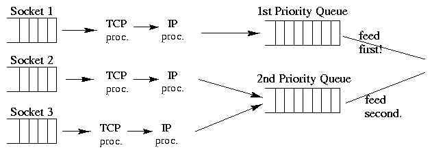
where the remaining data to be transferred is small. Figure
3 shows the flow of data in Linux after our
modifications.
Figure 3: Flow of data in Linux with SRPT-like scheduling (only
2 priority levels shown).
There are multiple priority queues and queue i may only drain if
queues 0 to i-1 are empty. The implementation is enabled by
building the Linux kernel with support for the user/kernel Netlink
Socket, QOS and Fair Queuing, and the Prio Pseudoscheduler and by
using the tc[6] user space tool. We also
modify Apache to use setsockopt calls to update the priority
of the socket as the remaining size of the transfer decreases. For
details on our implementation see
[19].
Synopsis of results:
Figure 2(a) shows results from the the static web
implementation under closed, open, and partly open workloads in a LAN
environment. Upon first glance, it is immediately clear that the
closed system response times are vastly different from the open
response times. In fact, the response times in the two systems are
orders of magnitude different under PS given a common system load.
Furthermore, SRPT provides little improvement in the closed system,
while providing dramatic improvement in the open system.
The third column of Figure 2(a) shows the results for
the partly-open system. Notice that when the mean number of requests
is small, the partly-open system behaves very much like the open
system. However, as the mean number of requests grows, the
partly-open system behaves more like a closed system. Thus, the
impact of scheduling (e.g. SRPT over PS) is highly dependent on the
number of requests in the partly-open system.
4.2 E-commerce site
Our second case study considers the database back-end server of an
e-commerce site, e.g. an online bookstore. We use a
PostgreSQL[32] database server running on a 2.4-GHz
Pentium 4 with 3GB RAM, running Linux 2.4, with a buffer pool of
2GB. The machine is equipped with two 120GB IDE drives, one used
for the database log and the other for the data. The workload is
generated by four client machines having similar specifications to
the database server connected via a network switch.
Workload generation: The workload
for the e-commerce case study is based on the TPC-W [46]
benchmark, which aims to model an online bookstore such as
Amazon.com. We build on the TPC-W kit
provided by the Pharm project [13]. The kit models a
closed system (in accordance with TPC-W guidelines) by creating
one process for each client in the closed system.
We extend the kit to also support an open system with Poisson
arrivals, and a partly-open system. We do so by creating a master
process that signals a client whenever it is time to make a new
request in the open system or to start a new session in the
partly-open system.
The master process repeats the following steps in a loop:
it sleeps for an exponential interarrival time, signals a client,
and draws the next inter-arrival time. The clients block waiting
for a signal from the master process. In the case of the open
system, after receiving the signal, the clients make one request
before they go back to blocking for the next signal. In the case
of the partly-open system, after receiving a signal, the clients
generate a session by executing the following steps in a loop: (1)
make one request; (2) flip a coin to decide whether to begin
blocking for a signal from the master process or to generate an
exponential think time and sleep for that time.
TPC-W consists of 16 different transaction types including the
"ShoppingCart" transaction, the "Payment" transaction, and
others. Statistics of our configuration are as shown:
|
| Database | Mean | Variability | Min | Max |
| size | size | (C2) | size | size |
| 3GB | 101 ms | 4 | 2 ms | 5s | |
Scheduling:
The bottleneck resource in our setup is the CPU, as observed in
[25]. The default
scheduling policy is therefore best described as PS, in accordance
with Linux CPU scheduling. Note that in this application, exact
service demands are not known, so SRPT cannot be implemented.
Thus, we experiment with PESJF and PELJF policies where the
expected service demand of a transaction is based on its type. The
"Bestseller" transaction, which makes up 10% of all requests,
has on average the largest service demand. Thus, we study
2-priority PESJF and PELJF policies where the "Bestseller"
transactions are "expected to be long" and all other
transactions are "expected to be short."
To implement the priorities needed for achieving PESJF and PELJF, we
modify our PostgreSQL server as follows.
We use the sched_setscheduler() system call to set the
scheduling class of a PostgreSQL process working on a high
priority transaction to "SCHED_RR," which marks a process as a
Linux real-time process. We leave the scheduling class of a low
priority process at the standard "SCHED_OTHER." Real-time
processing in Linux always has absolute, preemptive priority over
standard processes.
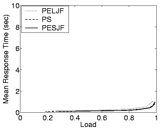
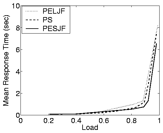
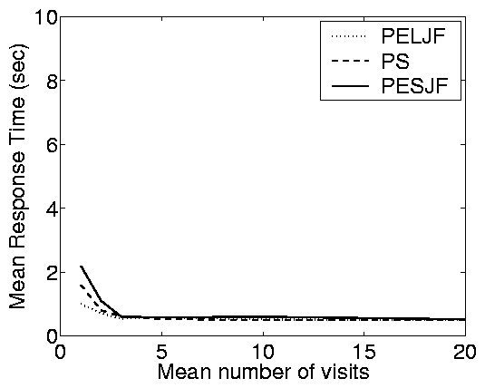
Synopsis of results:
Figure 2(b) shows results from the e-commerce
implementation described above. Again, the difference in response
times between the open and closed systems is immediately apparent -
the response times of the two systems differ by orders of magnitude.
Interestingly, because the variability of the service demands is much
smaller in this workload than in the static web workload, the impact
of scheduling in the open system is much smaller. This also can be
observed in the plot for the partly open system: even when the number
of requests is small, there is little difference between the response
times of the different scheduling policies.
4.3 Auctioning web site
Our third case study investigates an auctioning web site. This
case study uses simulation based on a trace from one of the
top-ten U.S. online auction sites.
Workload generation: For simulation-based case
studies we implement a simulator that
supports open, closed, and partly-open arrival processes which are
either created based on a trace or are generated from probability
distributions. For a trace-based arrival process the simulator
expects the same input files as the workload generator described in
Section 4.1. If no trace for the arrival process is
available the simulator alternatively offers (1) open system arrivals
following a Poisson process; (2) closed system arrivals with
exponential think times; (3) partly-open arrivals with session
arrivals following a Poisson process and think times within the
sessions being exponentially distributed. The service demands can
either be specified through a trace or one of several probability
distributions, including hyper-exponential distributions and more
general distributions.
For our case study involving an auctioning web site we use the
simulator and a trace containing the service demands obtained from
one of the top ten online auctioning sites in the US.
No data on the request arrival process is available.
The
characteristics of the service demands recorded in the trace are
summarized below:
|
| Number | Mean | Variability | Min | Max |
| of jobs | size | (C2) | size | size |
| 300000 | 0.09s | 9.19 | 0.01s | 50s | |
Scheduling: The policy used in a
web site serving dynamic content, such as an auctioning web site, is
best modeled by PS. To study the effect of scheduling in this
environment we additionally simulate FCFS and PSJF.
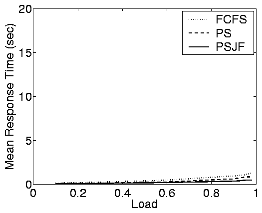
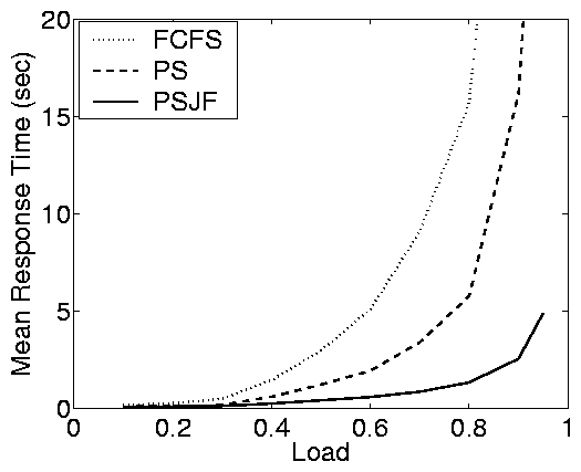
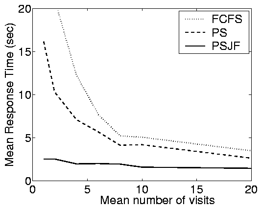
Synopsis of results:
Figure 2(c) shows results from the auctioning
trace-based case study described above. The plots here illustrate the
same properties that we observed in the case of the static web
implementation. In fact, the difference between the open and closed
response times is extreme, especially under FCFS. As a result, there
is more than a factor of ten improvement of PSJF over FCFS (for r > 0.7), whereas there is little difference in the closed system.
This effect can also be observed in the partly-open system, where for
a small number of requests per session the response times are
comparable to those in the open system and for a large number of
requests per session the response times are comparable to those in
the closed system. The actual convergence rate depends on the
variability of the service demands (C2). In particular, the
e-commerce case study (low C2) converges quickly, while the static
web and auctioning case studies (higher C2) converge more slowly.
|
 Closed System |
|
| |
|
 Open System |
|
| |
(a) Static web - Good WAN conditions
|
Closed System |
|
| |
|
 Open System |
|
| |
(b) Static web - Poor WAN conditions
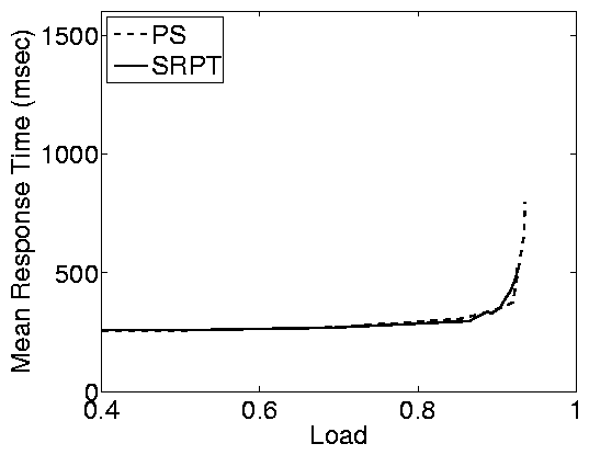
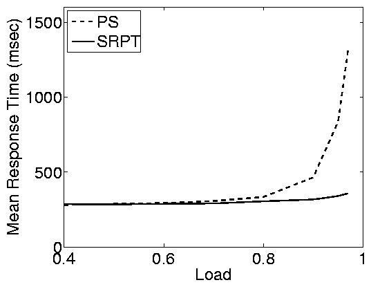
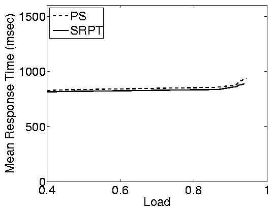
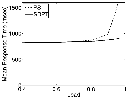
Figure 4: Effect of WAN conditions in the static web
case study. The top row shows results for good WAN conditions
(average RTT=50ms, loss rate=1%) and the bottom row shows results
for poor WAN conditions (average RTT=100ms, loss rate=4%). In
both cases the closed system has an MPL of 200. Note that, due to
network effects, the closed system cannot achieve a load of 1,
even when think time is zero. Under the settings we consider here,
the max achievable load is » 0.98.
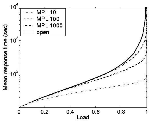
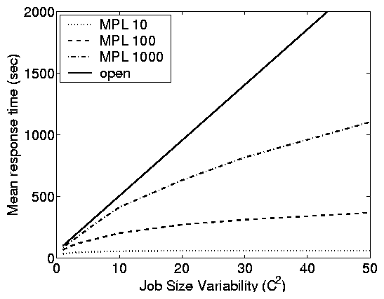
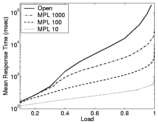
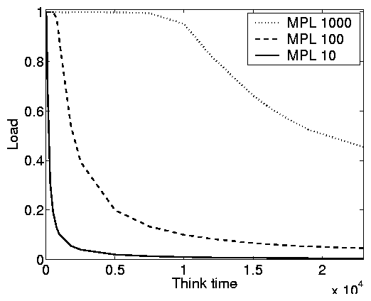
Figure 5: Open versus closed under FCFS. Model and trace-based simulation results showing
mean response time as a function of load and service demand
variability under FCFS scheduling. (a) and (b) use model based
simulation, while (c) uses trace-based simulation. In all cases, the solid line represents
an open system and the dashed lines represent closed systems with
different MPLs. The load is adjusted via the think time in the
closed system, and via the arrival rate in the open system. In the
model-based simulations, E[S] = 10. In (a) we fix C2=8 and in
(b) we fix r = 0.9.
4.4 Study of WAN effects
To study the effect of network conditions, we
return to the case of static web requests (Section 4.1),
but this time we include the emulation of network losses and delays in
the experiments.
Workload generation: The setup and
workload generation is identical to the case study of static web
requests (Section 4.1), except that we add
functionality for emulating WAN effects as follows. We implement a
separate module for the Linux kernel that can drop or delay
incoming and outgoing TCP packets (similarly to Dummynet
[34] for FreeBSD). More precisely, we change the
ip_rcv() and the ip_output() functions in the Linux
TCP-IP stack to intercept in- and out-going packets to create
losses and delays. In order to delay packets, we use the
add_timer() facility to schedule the transmission of delayed
packets. We recompile the kernel with HZ=1000 to get a
finer-grained millisecond timer resolution. In order to drop
packets, we use an independent, uniform random loss model which
can be configured to a specified probability, as in Dummynet.
Synopsis of results:
Figure 4 compares the response times of the closed
and the open systems under (a) relatively good WAN conditions
(50ms RTT and 1% loss rate) and under (b) poor WAN conditions
(100ms RTT and 4% loss rate). Note that results
for the partly-open system are not
shown due to space constraints; however the results parallel what is
shown in the closed and open systems.
We find that under WAN conditions the differences between the open
and closed systems are smaller (proportionally) than in a LAN
(Figure 2 (a)), however, they are still significant
for high server loads (load > 0.8). The reason that the
differences are smaller in WAN conditions is that response times
include network overheads (network delays and losses) in addition
to delays at the server. These overheads affect the response times
in the open and closed systems in the same way, causing the
proportional differences between open and closed systems to
shrink. For similar reasons, scheduling has less of an effect when
WAN effects are strong, even in the case of an open system. SRPT
improves significantly over PS only for high loads, and even then
the improvement is smaller than in a LAN.
5 Open versus closed systems
We have just seen the dramatic impact of the system model in
real-world case studies. We will now develop principles that help
explain both the differences between the open and closed system and
the impact of these differences with respect to scheduling. In
addition to the case studies that we have already discussed, we will
also use model-based simulations in order to provide more control
over parameters, such as job size variability, that are fixed in the
case studies.
Our study of the simple case of FCFS scheduling will illustrate three
principles that we will exploit when studying more complex policies.
Principle (i): For a given load, mean
response times are significantly lower in closed systems than in
open systems.
Principle (i) is maybe the most noticeable performance issue
differentiating open and closed systems in our case studies
(Figure 2). We bring further attention to this
principle in Figure 5 due to its importance
for the vast literature on capacity planning, which typically
relies on closed models, and hence may underestimate the resources
needed when an open model is more appropriate.
For fixed high loads, the response time under the closed system is
orders of magnitude lower than those for the open system.
While Schatte [36,37] has proven that, under
FCFS, the open system will always serve as an upper bound for the
response time of the closed system, the magnitude of the
difference in practical settings has not previously been studied.
Intuitively, this difference in mean response time between open
and closed systems is a consequence of the fixed MPL, N, in
closed systems, which limits the queue length seen in closed
systems to N even under very high load. By contrast, no such
limit exists for an open system.
Principle (ii): As the MPL grows,
closed systems become open, but convergence is slow for practical
purposes.
Principle (ii) is illustrated by Figure 5. We see
that as the MPL, N, increases from 10 to 100 to 1000, the curves
for the closed system approach the curves for the open system.
Schatte [36,37] proves formally that as N
grows to infinity, a closed FCFS queue converges to an open
M/GI/1/FCFS queue. What is interesting however, is how slowly
this convergence takes place. When the service demand has high
variability (C2), a closed system with an MPL of 1000 still has
much lower response times then the corresponding open system. Even
when the job service demands are lightly variable, an MPL of 500
is required for the closed system to achieve response times
comparable to the corresponding open system. Further, the
differences are more dramatic in the case-study results than in
the model-based simulations.
This principle impacts the choice of whether an open or closed system
model is appropriate. One might think that an open system is a
reasonable approximation for a closed system with a high MPL;
however, though this can be true in some cases, the closed and open
system models may still behave significantly differently if the
service demands are highly variable.
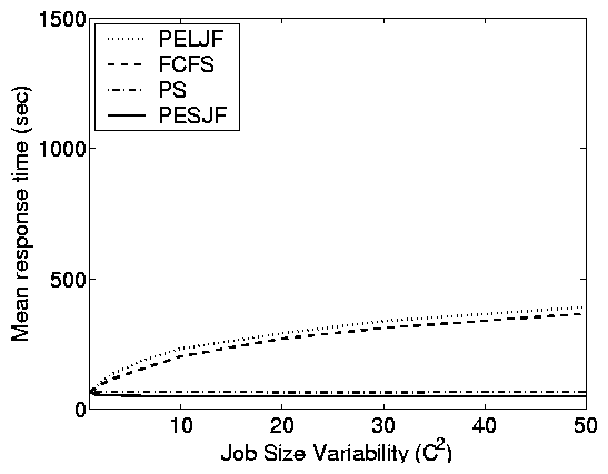
| |
(a) Response time vs. load
|
| |
|
| | | |
(b) Response time vs. variability
|
| |
Figure 6: Model-based simulation results illustrating
the different effects of scheduling in closed and open systems. In
the closed system the MPL is 100, and in both systems the service
demand distribution has mean 10. For the two figures in (a) C2
was fixed at 8 and in the two figures in (b) the load was fixed at
0.9.
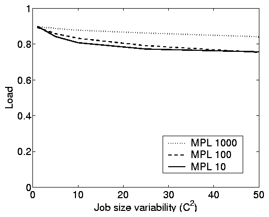
Principle (iii): While variability
has a large effect in open systems, the effect is much smaller in
closed systems.
This principle is difficult to see in the case-study figures (Figure
2) since each trace has a fixed variability. However, it
can be observed by comparing the magnitude of disparity between the
e-commerce site results (low variability) and the others (high
variability).
Using simulations, we can study this effect directly.
Figure 5(b) compares open and closed systems under a
fixed load r = 0.9, as a function of the service demand
variability C2. For an open system, we see that C2 directly
affects mean response time. This is to be expected since high
C2, under FCFS service, results in short jobs being stuck
behind long jobs, increasing mean response time. By contrast, for
the closed system with MPL 10, C2 has comparatively little
effect on mean response time. This is counterintuitive, but can be
explained by observing that for lower MPL there are fewer
short jobs stuck behind long jobs in a closed system, since the
number of jobs in the system (Nsystem) is bounded. As MPL is
increased, C2 can have more of an effect, since Nsystem
can be higher.
It is important to point out that by holding the load constant in
Figure 5(b), we are actually performing a
conservative comparison of open and closed systems. If we
didn't hold the load fixed as we changed C2, increasing C2
would result in a slight drop in
the load of the closed system as shown in Figure
7(b). This slight drop in load, would
cause a drop in response times for closed systems,
whereas there is no such effect in open systems.
|
(a) Think time vs. load
|
| |
|
(b) Variability vs. load
|
| |
Figure 7: Model-based simulation results illustrating
how the service demand variability, the MPL, and the think time
can affect the system load in a closed system. These plots use
FCFS scheduling, however results are parallel under other
scheduling policies.
5.2 The impact of scheduling
The value of scheduling in open systems is understood and cannot
be overstated. In open systems, there are order of magnitude
differences between the performance of scheduling policies because
scheduling can prevent small jobs from queueing behind large jobs.
In contrast, scheduling in closed systems is not well understood.
Principle (iv): While open systems
benefit significantly from scheduling with respect to response
time, closed systems improve much less.
Principle (v): Scheduling only
significantly improves response time in closed systems under very
specific parameter settings: moderate load (think times) and high
MPL.
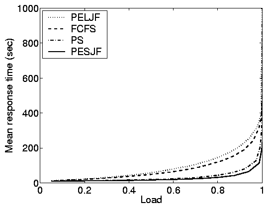
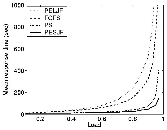
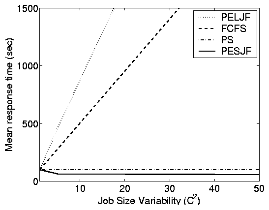
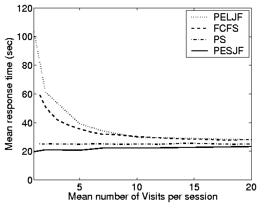
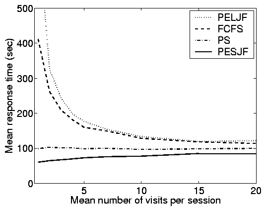
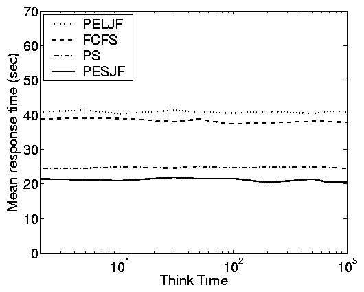
|
(c) Model-based simulation
|
Figure 8: Model and implementation-based results for
the partly-open system. (a) and (b) are model-based simulations
showing mean response time as a function of the expected number of
requests per session. (c) and (d) show the mean response time as a
function of the think time, for a fixed load. In
(a)-(c), E[S]=10 and C2=8. In (c) and (d), we fix r = 0.6
and p=0.75, which yields and average of 4 requests per session.
Figure 2 illustrates the fundamentally different
behavior of mean response time in the open and closed systems in
realistic settings. In Figure 6, we further
study this difference as a function of (a) load and (b)
variability using simulations. Under the open system, as load
increases, the disparity between the response times of the
scheduling policies grows, eventually differing by orders of
magnitude. In contrast, at both high and low loads in the closed
system, the scheduling policies all perform similarly; only at
moderate loads is there a significant difference between the
policies - and even here the differences are only a factor of
2.5. Another interesting point is that, whereas for FCFS the mean
response time of an open system bounded that in the corresponding
closed system from above, this does not hold for other policies
such as PESJF, where the open system can result in lower response
times than the closed system.
We can build intuition for the limited effects of scheduling in
closed systems by first considering a closed feedback loop with no
think time. In such a system, surprisingly, the scheduling done at
the queue is inconsequential - all work conserving scheduling
policies perform equivalently. To see why, note that in a closed
system Little's Law states that N=X E[T], where N is the
constant MPL across policies. We will now explain why X is
constant across all work conserving scheduling policies (when
think time is 0), and hence it will follow that E[T] is also
constant across scheduling policies. X is the long-run average
rate of completions. Since a new job is only created when a job
completes, over a long period of time, all work conserving
scheduling policies will complete the same set of jobs plus or
minus the initial set N. As time goes to infinity, the initial
set N becomes unimportant; hence X is constant. This argument
does not hold for open systems because for open systems Little's
Law states that E[N] = lE[T], and E[N] is not constant
across scheduling policies.
Under closed systems with think time, we now allow a varying
number of jobs in the queue, and thus there is some difference
between scheduling policies. However, as think time grows, load
becomes small and so scheduling has less effect.
A very subtle effect, not yet mentioned, is that in a closed
system the scheduling policy actually affects the throughput, and
hence the load. "Good" policies, like PESJF, increase
throughput, and hence load, slightly (less than 10%). Had we
captured this effect (rather than holding the load fixed), the
scheduling policies in the closed system would have appeared even
closer, resulting in even starker differences between the closed
and open systems.
The impact of Principles (iv) and (v) is clear. For closed
systems, scheduling provides small improvement across all
loads, but can only result in substantial improvement when load
(think time) is moderate. In contrast, scheduling always
provides substantial improvements for open systems.
Principle (vi): Scheduling can limit
the effect of variability in both open and closed systems.
For both the open and closed systems, better scheduling (PS and
PESJF) helps combat the effect of increasing variability, as seen in
Figure 6. The
improvement; however, is less dramatic for closed systems due to
Principle (iii) in Section 5.1, which tells us
that variability has less of an effect on closed systems in
general.
6 Partly-open systems
In this section, we discuss a partly-open model that (a) serves as
a more realistic system model for many applications; and (b) helps
illustrate when a "purely" open or closed system is a good
approximation of user behavior. We focus on the effects of the
mean number of requests per session and the think time because the
other parameters, e.g. load and job size variability, have similar
effects to those observed in Sections 5.1 and
5.2. Throughout the section, we fix the load of the
partly-open system by adjusting the arrival rate, l. Note
that, in contrast to the closed model, adjusting the think time of
the partly-open model has no impact on the load.
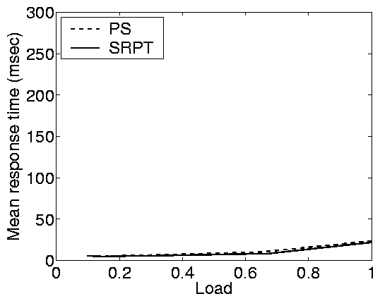
Principle (vii): A partly-open system
behaves similarly to an open system when the expected number of
requests per session is small ( £ 5 as a rule-of-thumb) and
similarly to a closed system when the expected number of requests
per session is large ( ³ 10 as a rule-of-thumb).
Principle (vii) is illustrated clearly in the case study results
shown in Figure 2 and in the simulation results shown
in Figure 8(a). When the mean number of requests
per session is 1 we have a significant separation between the
response time under the scheduling policies, as in open systems.
However, when the mean number of requests per session is large, we
have comparatively little separation between the response times of
the scheduling policies; as in closed systems. Figures
2 and 8(a) are just a few examples of
the range of configurations we studied, and across a wide range of
parameters, the point where the separation between the performance
of scheduling policies becomes small is, as a rule-of-thumb,
around 10 requests per session. Note however that this point can
range anywhere between 5 and 20 requests per session as C2 ranges
from 4 to 49 respectively.
We will demonstrate in Section 7 how to use this rule-of-thumb
as a guideline for determining whether a purely open or purely closed
workload generator is most suitable, or whether a partly-open generator is
necessary.
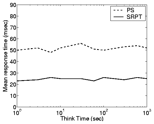
Principle (viii): In a partly-open
system, think time has little effect on mean response
time.
Figure 8 illustrates Principle (viii). We find that
the think time in the partly-open system does not affect the mean
response time or load of the system under any of these policies.
This observation holds across all partly-open systems we have
investigated (regardless of the number of requests per session),
including the case-studies described in Section 4.
Principle (viii) may seem surprising at first, but for PS and FCFS
scheduling it can be shown formally under product-form workload
assumptions. Intuitively, we can observe that changing the think
time in the partly-open system has no effect on the load because
the same amount of work must be processed. To change the load, we
must adjust either the number of requests per session or the arrival
rate. The only effect of think time is to add small correlations
into the arrival stream.
7 Choosing a system model
The previous sections brought to light vast differences in system
performance depending on whether the workload generator follows an
open or closed system model. A direct consequence is that the
accuracy of performance evaluation depends on accurately modeling the
underlying system as either open, closed, or partly-open.
A safe way out would be to choose a partly-open system model,
since it both matches the typical user behavior in many
applications and generalizes the open and closed system models -
depending on the parameters it can behave more like an open or
more like a closed system. However, as Table 1
illustrates, available workload generators often support only
either closed or open system models. This motivates a fundamental
questions for workload modeling: "Given a particular
workload, is a purely open or purely closed system model more
accurate for the workload? When is a partly-open system model
necessary?"
In the remainder of this section we illustrate how our eight principles
might be used to answer this
question for various web workloads.
Our basic method is as follows.
For a given system we follow these steps:
- Collect traces from the system.
- Construct a partly-open model for the system,
since the partly-open model is the most general and accurate. In
particular, obtain the relevant parameters for the partly-open
model.
- For the partly-open model, decide whether
an open or a closed model is appropriate, or if
the partly-open model is necessary.
Table 2 summarizes the traces we collected as part of
Step 1. Our trace collection spans many different types of sites,
including busy commercial sites, sites of major sporting events,
sites of research institutes, and an online gaming site.
|
| Type of site | Date | Total #Req. |
| 1 | Large corporate web site | Feb'01 | 1609799 |
| 2 | CMU web server [3] | Nov'01 | 90570 |
| 3 | Online department store | June'00 | 891366 |
| 4 | Science institute (USGS[1]) | Nov'02 | 107078 |
| 5 | Online gaming site [50] | May'04 | 45778 |
| 6 | Financial service provider | Aug'00 | 275786 |
| 7 | Supercomputing web site [4] | May'04 | 82566 |
| 8 | Kasparov-DeepBlue match | May'97 | 580068 |
| 9 | Site seeing "slashdot effect" | Feb'99 | 194968 |
| 10 | Soccer world cup [21] | Jul'98 | 4606052 | |
|
Table 2: A summary table of the studied web
traces.
We next model each site as a partly-open system. According to
Principles (vii) and (viii) the most relevant parameter of a
partly-open system model is the number of requests issued in a user
session. Other parameters such as the think time between
successive requests in a session are of lesser importance.
Determining the average number of requests per user session for a
web site requires identifying user sessions in the corresponding
web trace. While there is no 100% accurate way to do this, we
employ some common estimation techniques [8,26].
First, each source IP address in a trace is taken to represent a
different user. Second, session boundaries are determined by a
period of inactivity by the user, i.e. a period of time during
which no requests from the corresponding IP address are received.
Typically, this is accomplished by ending a session whenever there
is a period of inactivity larger than timeout threshold t. In
some cases, web sites themselves enforce such a threshold;
however, more typically t must be estimated.
We consider two different ways of estimating t. The first one
is to use a defacto standard value for t, which is 1800s (30
min) [26]. The second method is to estimate t from the
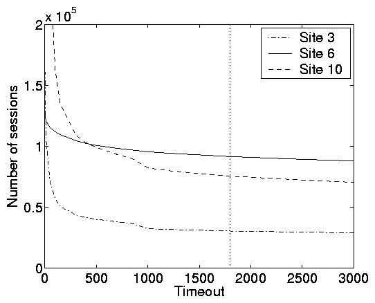
traces themselves by studying the derivative of how t affects the total
number of sessions in the trace. We illustrate this latter method for a few
representative traces in Figure 9(a). Notice that as
the threshold increases from 1-100s the number of sessions
decreases quickly; whereas from 1000s on, the decrease is much
smaller.
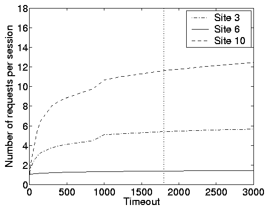
Furthermore, Figure 9(b) shows that with respect to the
number of requests, stabilization is also reached at t > 1000s.
Hence we adopt t = 1800s in what follows.
 (a) Number of sessions vs Timeout length
|
|
(b) Number of requests vs Timeout length
|
| |
Figure 9: Choosing a system model. Statistics for 3 representative web traces
(sites 3, 6, and 10) illustrating (a) the number of user sessions
as a function of the timeout threshold and (b) the expected number
of requests per session as a function of the timeout threshold.
The vertical line on each plot corresponds to a timeout of 1800s.
From these plots we can conclude that an open model is appropriate
for site 6, a closed model is appropriate for site 10, and neither
an open or a closed is appropriate for site 3.
The mean number of requests per session when t = 1800s is
summarized below for all traces:
|
| Site | 1 | 2 | 3 | 4 | 5 |
| Requests per session | 2.4 | 1.8 | 5.4 | 3.6 | 12.9 | |
| Site | 6 | 7 | 8 | 9 | 10 |
| Requests per session | 1.4 | 6.0 | 2.4 | 1.2 | 11.6 | |
|
The table indicates that the average number of requests
for web sessions varies largely depending on the site, ranging
from less than 2 requests per session to almost 13. Interestingly,
even for similar types of web sites the number of requests can
vary considerably. For example sites 8 and 10 are both web sites
of sporting events (a chess tournament and a soccer tournament),
but the number of requests per session is quite low (2.4) in one
case, while quite high (11.6) in the other. Similarly, sites 2, 4,
and 7 are all web sites of scientific institutes but the number of
requests per sessions varies from 1.8 to 6.
Using the rule of thumb in principle (vii), we can conclude that
neither the open nor the closed system model accurately represents
all the sites. For sites 1, 2, 4, 6, 8, and 9 an open system model
is accurate; whereas a closed system model is accurate for the sites
5 and 10. Further, it is not clear whether an open or closed model is
appropriate for sites 3 and 7.
Observe that the web trace of site 10 is the same dataset used to drive the
static web case study in Figure 2. In Figure 2, we
observed a large difference between the response times in an open and a closed
system model. In this section we found that site 10 resembles more a closed system than an
open system. Based on the results in Figure 2, it is important that one doesn't
assume that the results for the closed model apply to the open model.
8 Prior Work
Work explicitly comparing open and closed system models is
primarily limited to FCFS queues. Bondi and Whitt
[11] study a general network of FCFS queues and
conclude that the effect of service variability, though dominant
in open systems, is almost inconsequential in closed systems
(provided the MPL is not too large). We corroborate this
principle and illustrate the magnitude of its impact in real-world
systems. Schatte [36,37] studies a single FCFS
queue in a closed loop with think time. In this model, Schatte
proves that, as the MPL grows to infinity, the closed system
converges monotonically to an open system. This result provides a
fundamental understanding of the effect of the MPL parameter;
however the rate of this convergence, which is important when
choosing between open and closed system models, is not understood.
We evaluate the rate of convergence in real-world systems.
Though these theoretical results provide useful intuition about
the differences between open and closed systems, theoretical
results alone cannot evaluate the effects of factors such as trace
driven job service demand distributions, correlations,
implementation overheads, and size-based scheduling policies.
Hence, simulation and implementation-based studies such as the
current paper are needed.
9 Conclusion
This paper provides eight simple principles that function to explain
the differences in behavior of closed, open, and partly-open systems
and validates these principles via trace-based simulation and
real-world implementation. The more intuitive of these principles
point out that response times under closed systems are typically
lower than in the corresponding open system with equal load, and that
as MPL increases, closed systems approach open ones. Less obviously,
our principles point out that: (a) the magnitude of the difference in
response times between closed and open systems can be very large,
even under moderate load; (b) the convergence of closed to open as
MPL grows is slow, especially when service demand variability (C2)
is high; and (c) scheduling is far more beneficial in open systems
than in closed ones. We also compare the partly-open model with the
open and closed models. We illustrate the strong effect of the
number of requests per session and C2 on the behavior of the
partly-open model, and the surprisingly weak effect of think time.
These principles underscore the importance of choosing the
appropriate system model. For example, in capacity planning for
an open system, choosing a workload generator based on a closed
model can greatly underestimate response times and
underestimate the benefits of scheduling.
All of this is particularly relevant in the context of web
applications, where the arrival process at a web site is best modeled
by a partly-open system. Yet, most web workload generators are
either strictly open or strictly closed. Our findings provide
guidelines for choosing whether an open or closed model is the better
approximation based on characteristics of the workload. A high
number of simultaneous users (more than 1000) suggests an open model,
but a high number of requests per session (more than 10) suggests a
closed model. Both these cutoffs are affected by service demand
variability: highly variable demands requires larger cutoffs.
Contrary to popular belief, it turns out that think times are
irrelevant to the choice of an open or closed model since they only
affect the load. We also find that WAN conditions (losses and delays)
in Web settings lessen the difference between closed and open models,
although these differences are still noticeable.
Once it has been determined whether a closed or open model is a
better approximation, that in turn provides a guideline for the
effectiveness of scheduling. Understanding the appropriate
system model is essential to understanding the impact of
scheduling. Scheduling is most effective in open systems, but can
have moderate impact in closed systems when both the load is
moderate (roughly 0.7-0.85) and C2 is high.
In conclusion, while much emphasis has been placed in research on
accurately representing workload parameters such as service demand
distribution, think time, locality, etc, we have illustrated that
similar attention needs to be placed on accurately representing
the system itself as either closed, open, or partly-open. We have
taken a first step toward this end by providing guidelines for
choosing a system model and by creating tools and workload
generators versatile enough to support all three system models.
We hope that this work will encourage others to design workload
generators that allow flexibility in the underlying system model.
10 Acknowledgments
We would like to thank Arun Iyengar, Erich Nahum, Paul Dantzig, Luis von Ahn, and
Chad Vizino for providing access to the logs we used in Section 4.3 and Section 7.
This work was supported by an IBM PhD fellowship, NSF grants CCR-0133077, CCR-0311383,
and CCR-0313148, and by IBM via TTC grant 2005-2006.
References
- [1]
-
The U.S. Geological Survey.
http://www.usgs.gov.
- [2]
-
Webjamma world wide web traffic analysis tools.
http://research.cs.vt.edu/chitra/webjamma.html.
- [3]
-
Carnegie Mellon University, School of Computer Science.
http://www.cs.cmu.edu/, 2005.
- [4]
-
The Pittsburgh Supercomputing Center (PSC).
http://www.psc.edu/, 2005.
- [5]
-
J. Almeida and P. Cao.
Wisconsin proxy benchmark 1.0.
http://www.cs.wisc.edu/cao/wpb1.0.html, 1998.
- [6]
-
W. Almesberger.
Linux network traffic control - implementation overview.
http://diffserv.sourceforge.net, 1999.
- [7]
-
C. Amza, E. Cecchet, A. Chanda, A. Cox, S. Elnikety, R. Gil, J. Marguerite,
K. Rajamani, and W. Zwaenepoel.
Specification and implementation of dynamic web site benchmarks.
In Workshop on Workload Characterization, 2002.
- [8]
-
M. Arlitt.
Characterizing web user sessions.
SIGMETRICS Perform. Eval. Rev., 28(2):50-63, 2000.
- [9]
-
G. Banga and P. Druschel.
Measuring the capacity of a web server under realistic loads.
World Wide Web, 2(1-2):69-83, 1999.
- [10]
-
P. Barford and M. Crovella.
The surge traffic generator: Generating representative web workloads
for network and server performance evaluation.
In In Proc. of the ACM SIGMETRICS, 1998.
- [11]
-
A. B. Bondi and W. Whitt.
The influence of service-time variability in a closed network of
queues.
Perf. Eval., 6:219-234, 1986.
- [12]
-
Bradford L. Barrett.
The Webalizer log file analysis program.
http://www.mrunix.net/webalizer, 2005.
- [13]
-
T. Cain, M. Martin, T. Heil, E. Weglarz, and T. Bezenek.
Java TPC-W implementation.
http://www.ece.wisc.edu/
~ pharm/tpcw.shtml, 2000.
- [14]
-
R. Chinchilla, J. Hoag, D. Koonce, H. Kruse, S. Ostermann, and Y. Wang.
The trafgen traffic generator.
In Proc. of Int. Conf. on Telecommunication Sys., Mod. and Anal.
(ICTSM10), 2002.
- [15]
-
M. Crovella, R. Frangioso, and M. Harchol-Balter.
Connection scheduling in web servers.
In USENIX Symposium on Internet Technologies and Systems,
October 1999.
- [16]
-
A. Feldmann, A. C. Gilbert, P. Huang, and W. Willinger.
Dynamics of IP traffic: A study of the role of variability and the
impact of control.
In Proc. ACM Sigcomm, 1999.
- [17]
-
J. Fulmer.
Siege.
http://joedog.org/siege.
- [18]
-
S. Gigandet, A. Sudarsanam, and A. Aggarwal.
The inktomi climate lab: an integrated environment for analyzing and
simulating customer network traffic.
In Proc. ACM SIGCOMM Workshop on Int. Meas., pages 183-187,
2001.
- [19]
-
M. Harchol-Balter, B. Schroeder, M. Agrawal, and N. Bansal.
Size-based scheduling to improve web performance.
ACM Transactions on Computer Systems, 21(2), May 2003.
- [20]
-
P. E. Heegaard.
Gensyn - generator of synthetic internet traffic.
http://
www.item.ntnu.no/ ~ poulh/GenSyn/gensyn.html.
- [21]
-
ITA.
The Internet traffic archives.
Available at
http://town.hall.org/Archives/pub/ITA/, 2002.
- [22]
-
K. Kant, V. Tewari, and R. Iyer.
GEIST: Generator of e-commerce and internet server traffic.
In Proc. of Int. Symposium on Performance Analysis of Systems
and Software, 2001.
- [23]
-
Z. Liu, N. Niclausse, and C. Jalpa-Villanueva.
Traffic model and performance evaluation of web servers.
Performance Evaluation, 46(2-3):77-100, 2001.
- [24]
-
B. A. Mah, P. E. Sholander, L. Martinez, and L. Tolendino.
Ipb: An internet protocol benchmark using simulated traffic.
In MASCOTS 1998, pages 77-84, 1998.
- [25]
-
D. T. McWherter, B. Schroeder, A. Ailamaki, and M. Harchol-Balter.
Priority mechanisms for OLTP and transactional web applications.
In Int. Conf. on Data Engineering, 2004.
- [26]
-
D. Menasce and V. Almeida.
Scaling for E-Buisness: technologies, models, performance, and
capacity planning.
Prentice Hall, 2000.
- [27]
-
Microsoft IIS 6.0 Resource Kit Tools.
Microsoft Web Capacity Analysis Tool (WCAT) version 5.2.
- [28]
-
Microsoft TechNet.
Ms web application stress tool (WAST).
- [29]
-
Mindcraft.
The AuthMark benchmark.
http://www.mindcraft.com
/authmark/.
- [30]
-
D. Mosberger and T. Jin.
httperf: A tool for measuring web server performance.
Performance Evaluation Review, 26(3), 1998.
- [31]
-
E. Nahum, M. Rosu, S. Seshan, and J. Almeida.
The effects of wide-area conditions on WWW server performance.
In Proc of ACM SIGMETRICS, pages 257-267, 2001.
- [32]
-
PostgreSQL.
http://www.postgresql.org.
- [33]
-
M. Rakwat and A. Kshemkayani.
SWIFT: Scheduling in web servers for fast response time.
In Symp. on Net. Comp. and App., April 2003.
- [34]
-
L. Rizzo.
Dummynet: a simple approach to the evaluation of network protocols.
ACM Comp. Comm. Review, 27(1), 1997.
- [35]
-
A. Rousskov and D. Wessels.
High performance benchmarking with web polygraph.
Software - Practice and Experience, 1:1-10, 2003.
- [36]
-
P. Schatte.
On conditional busy periods in n/M/GI/1 queues.
Math. Operationsforsh. u. Statist. ser. Optimization, 14, 1983.
- [37]
-
P. Schatte.
The M/GI/1 queue as limit of closed queueing systems.
Math. Operationsforsh. u. Statist. ser. Optimization,
15:161-165, 1984.
- [38]
-
sourceforge.net.
Deluge - a web site stress test tool.
http://deluge.sourceforge.net/.
- [39]
-
sourceforge.net.
Hammerhead 2 - web testing tool.
http://hammerhead.sourceforge.net/.
- [40]
-
Standard Performance Evaluation Corporation.
SFS97_R1 (3.0).
http://www.specbench.org/osg/web99/.
- [41]
-
Standard Performance Evaluation Corporation.
SPECJ2EE.
http://www.specbench.org/osg/web99/.
- [42]
-
Standard Performance Evaluation Corporation.
SPECmail2001.
http://www.specbench.org/osg/web99/.
- [43]
-
Standard Performance Evaluation Corporation.
SPECweb99.
http://www.specbench.org/osg/web99/.
- [44]
-
W. Tang, Y. Fu, L. Cherkasova, and A. Vahdat.
Medisyn: A synthetic streaming media service workload generator.
In Proceedings of 13th NOSSDAV, 2003.
- [45]
-
Transaction Processing Performance Council.
TPC benchmark C.
Number Revision 5.1.0, December 2002.
- [46]
-
Transaction Processing Performance Council.
TPC benchmark W (web commerce).
Number Revision 1.8, February 2002.
- [47]
-
G. Trent and M. Sake.
WebStone: The first generation in HTTP server benchmarking.
http://www.mindcraft.com/webstone/paper.html.
- [48]
-
VeriTest.
Netbench 7.0.3.
http://www.etestinglabs.
com/benchmarks/netbench/.
- [49]
-
VeriTest.
Webbench 5.0.
http://www.etestinglabs.
com/benchmarks/webbench/.
- [50]
-
L. von Ahn and L. Dabbish.
Labeling images with a computer game.
In CHI '04: Proceedings of the SIGCHI conference on Human
factors in computing systems, pages 319-326, 2004.
- [51]
-
B. L. Worthington, G. R. Ganger, and Y. N. Patt.
Scheduling algorithms for modern disk drives.
In Proc. of Sigmetrics, 1994.
- [52]
-
M. Yuksel, B. Sikdar, K. S. Vastola, and B. Szymanski.
Workload generation for ns simulations of wide area networks and the
internet.
In Proc. of Comm. Net. and Dist. Sys. Mod. and Sim., 2000.
Footnotes:
1Note that we choose a Poisson arrival process
(i.e. exponential inter-arrival times) and exponential think
times in order to allow the open and closed systems to be as
parallel as possible. This setting underestimates the differences
between the systems when more bursty arrival processes are used.
File translated from
TEX
by
TTH,
version 3.73.
On 29 Mar 2006, 18:12.
|
|
|