|
||||||||||||||
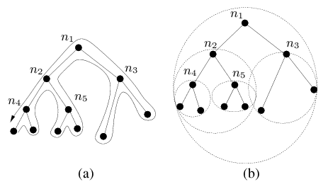
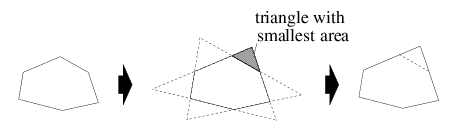
The convex hull for a set of points is the minimal convex polygon that contains all the points; it is minimal because the convex hull will be contained in any convex polygon that contains the given points. The hull is represented as a set of points (its vertices), and this set could be arbitrarily large. To ensure that the convex hulls use only O(1) storage instead of O(N) storage, where N is the network size, we can limit the number of vertices for a convex hull to a maximum of r points. To reduce a convex hull with s vertices to a smaller one with s - 1 points, we can project the boundary lines to form an adjacent triangle at every face. We pick the smallest triangle in this set of s triangles and add that triangle to the hull as illustrated in Figure 2. Limiting the number of points on the convex hulls allows us to save storage, but the resulting hulls will be larger and this increases the probability that the hulls of two siblings nodes in a tree will intersect. Intersections between convex hulls are undesirable because they introduce ambiguity in the routing process and make it less efficient. However, our experiments (described in Section 5) show that routing behavior is not affected by using as few as 5 points to represent a hull. 3.2 Overview of RoutingGDSTR forwards packets using simple greedy forwarding whenever possible. It switches to forwarding based on a hull tree only to route packets around ``voids,'' and escape from a local minimum. It switches back to greedy forwarding as soon as it is feasible to do so. When a packet reaches a local minimum, there are the following possibilities:
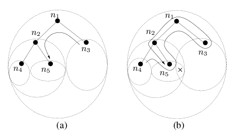
Routing using hull trees is illustrated in Figure 3. Figure 3(a) shows what happens when node n3 sends a packet to node n5: since n5 is not in n3's convex hull, the packet will be sent first to n1, and from there to n2, since its convex hull contains the destination. Figure 3(b) illustrates a more complex example involving an undeliverable packet. Suppose node n4 sends a message to an unreachable destination x, and initially this packet is routed greedily to n2, and then to n5, which is a local minimum. At this point n5 records itself in the packet and switches to routing in tree forwarding mode. The packet is forwarded on the subtree consisting of the nodes with hulls that contain the destination (which in our example are the nodes n1, n2, n3 and n5). The packet is first sent to the parent node n2 and from there to n1. The destination is contained in the convex hulls of both of n1's child nodes, but since the packet was received from n2, it is forwarded to n3. After forwarding over subtrees of n3 (not shown on the diagram), the packet is returned to n1, which forwards it to n2, its first child whose convex hull contains the packet. n2 forwards the packet to n5. At this point n5 sees that it was the originator of the tree traversal and hence concludes that the packet is undeliverable.
3.3 Optimization for Undeliverable PacketsThe example in Figure 3(b) illustrates that undeliverable packets will unfortunately always be routed to the root of a hull tree. For applications like data-centric sensor networks where the destination of packets often do not correspond to actual nodes, this situation is unacceptable. The problem arises because, during tree traversal, a node that receives a packet from its last child node does not know if there is any other convex hull in another part of the tree that contains the destination and has no choice but to forward the packet to the parent node.
To remedy this situation, we maintain additional information in the
tree to allow a node to decide if the destination of a packet could
possibly be in a distant branch of the tree reachable only by
forwarding the packet up the tree. In addition to its convex hull,
each node maintains information about the set of convex hulls With this additional information, a node that receives a packet from its last child during tree traversal will check if any of its conflict hulls contain the destination. If not, it will forward the packet to its first child instead of the parent. Effectively, the conflict hulls allow us to prune some nodes at the root of the routing subtree during tree traversal. 3.4 Using Multiple TreesUsing a single tree as the basis of routing is inherently fragile. If the root node fails, the entire tree may collapse and have to be rebuilt, and while this is happening, routing will not work well. GDSTR provides some degree of resilience to such network changes by maintaining a set of k hull trees, each of which is uniquely defined by its root node. With multiple trees, a tree must be chosen when a packet switches from greedy forwarding to tree forwarding mode. We studied a number of heuristics [19] and found that following simple heuristic works best:
3.5 Routing Algorithm
The following is a more precise description of GDSTR that incorporates
the use of multiple trees and the set of conflict hulls
Algorithm (GDSTR) When a node v receives packet p for
destination node t from a neighboring node
u, do:
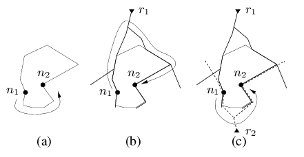
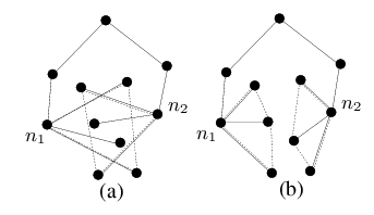
The correctness of this algorithm follows from the fact that the geometric properties of the routing subtree will ensure that a packet will eventually visit every node that can possibly be its destination. Termination is guaranteed because |(p.nmin)t| is strictly decreasing while a packet is in greedy forwarding mode; and if a packet is not deliverable, it will eventually return to the anchor node nanchor in tree traversal mode [19]. 3.6 Why and How Hull Trees WorkThe common wisdom about spanning trees is that they result in low total performance: routes can only use tree links, leaving the majority of links idle. However, this drawback does not apply to GDSTR for two reasons. The first reason is that GDSTR uses tree routing only when greedy geographic forwarding encounters a dead end. Furthermore GDSTR switches back to greedy forwarding as soon as possible. Thus typically only a small fraction of hops use tree routing and few packets are routed through the root nodes of the hull trees. Since greedy forwarding yields good stretch when it works [34], GDSTR provides good overall performance. The second reason GDSTR performs well is that it does a good job of routing around voids. GDSTR achieves this by using hull trees that are rooted at the extremities of the network, which allows it to find routes that conform closely to the voids. Figure 4 illustrates this point. Suppose that node n1 in Figure 4(a) needs to route a packet around a void to n2. A face routing algorithm is likely to have a face exactly corresponding to the void, and must choose between routing clockwise or counter-clockwise. In this example, the optimal choice is counterclockwise. While having some local face information allows a face routing algorithm to pick the optimal direction fairly often [20], local information alone cannot guarantee that the optimal routing direction will be picked when the void is large. Suppose GDSTR is the routing algorithm and has one hull tree rooted at r1. As illustrated in Figure 4(b), n1 would be forced to route clockwise. However, with another tree rooted at r2, at the opposite end of the network, n1 is presented with the other choice as well, as illustrated in Figure 4(c). This example demonstrates how two trees can effectively ``approximate'' a planar face. This insight into how the hull trees work also explains the expected performance trade off between GDSTR and face routing algorithms. Face routing techniques are able to traverse voids in a wireless routing topology relatively efficiently. The key issue is that they often do not have sufficient information to choose the optimal forwarding direction and it can be very costly when they make a bad choice. It turns out that with GDSTR where there are at least two extremally-rooted trees, the simple heuristic of choosing the tree with a root that is nearest to the destination often allows GDSTR to choose the more favorable forwarding direction around a void (because it effectively has global information). For sparse networks with large voids, GDSTR is thus able to perform significantly better than geographic face routing algorithms. For dense networks, the voids tend to be small and it generally does not matter which forwarding direction is picked. Because hull trees are not able to approximate voids quite as well as planar faces, face routing is expected to achieve slightly better stretch than GDSTR in such cases. 3.7 Building and Maintaining Hull TreesThis section explains how we build and maintain hull trees. Choosing Root Nodes. Since our goal is to use hull trees to ``approximate'' voids, we want the roots of the k hull trees as far apart as possible. To achieve this, we choose k rays in different directions, rooted at the origin, and the roots are the nodes whose projections onto these rays are farthest from the origin. If there are multiple extremal nodes, we break ties by imposing a global ordering on the node identifiers. For example, to maintain two trees, we can use one rooted at the node with the maximal x coordinate and the other rooted at the node with the minimal x coordinate. Each node broadcasts a keepalive message periodically to inform its neighbors of its location. The node includes in each message its view of the root of each tree and its distance in both hop count and path distance from each root. Through these exchanges, all the nodes will eventually come to a consensus as to which nodes should be roots; each node will also know both its hop count and total path distance from the root. Spanning Tree Algorithm. GDSTR will work correctly with any distributed spanning tree. However, routing performance will be best if there is minimal overlap among the convex hulls of different tree branches. Intuitively, we want trees that are geographically ``compact.'' Figure 5 illustrates this idea. While the nodes in both Figures 5(a) and 5(b) are the same, the tree configuration in Figure 5(a) creates an undesirable intersection in the hulls for nodes n1 and n2. From these examples, it is clear that we want to build trees that cluster nearby nodes in the same subtree. In addition, we want to be able to route from the root of the tree to all the nodes in the network in a small number of hops, since this will likely reduce the routing hop count. After evaluating a number of spanning tree algorithms, we found that the minimal-path tree seems to work best. The minimal-path tree is constructed by having each node choose the neighbor with the minimal path distance to the root as its parent (and updating its path distance accordingly). The details and simulation results for the other spanning tree algorithms are contained in [19]. Building Hull Trees. Once the tree has been formed, each node broadcasts its chosen parent node as well as its convex hull. To compute its convex hull, a node determines the minimal convex hull that contains the union of the convex hulls of its children in that tree. The convex hull for a set of points can be computed in O(n log n) operations using the Graham's Scan algorithm [6].
Once the root acquires hulls from all its children, the final step is
for each node is to determine the set of conflict hulls Maintenance & Repair. We use the same algorithm to repair a tree when nodes fail. If the mean inter-message interval is T seconds, even in the worst case where the root of a tree fails, a hull tree can be restored within 3TD seconds. To speed up tree repair and recovery, we can trigger immediate transmissions in place of regular messages when a node failure is detected. A node concludes that a neighbor has failed when it does not hear from it after a pre-determined multiple of the keepalive message interval. If the failed node is a child, a node will reduce and update its convex hull; if the failed node is a parent, a node will choose a new parent. In either case, it sends the new information in its next keepalive message. When the (new or old) parent hears about the changes, it will update its state accordingly. Hence, it is straightforward to update the routing state when anything changes in the system. When a node hears the keepalive message from a neighbor, it updates its own state and the information that it broadcasts in its subsequent keepalive message. If nothing changes, a node does not need to update anything. In fact, a node only has to broadcast its hull tree information when there are changes to the state of its hull trees. If nothing changes after the same hull tree information has been sent for several rounds, subsequent keepalive messages will contain only the node's identifier and location. When there is a change in its hull tree information, a node resumes broadcasting its hull tree information for another few rounds. Assumptions. The spanning tree algorithm makes few assumptions about radio behavior. The only requirement is that nodes must agree about whether they are neighbors. GDSTR is also robust to location errors [29], because if a node has a wrong location, the hulls in its part of the hull trees will grow to include the node's wrong location. When greedy routing to that node hits a dead end, GDSTR's tree traversal will eventually route to the tree branch that includes the node because of the large hull.
|
|||||||||||||
|
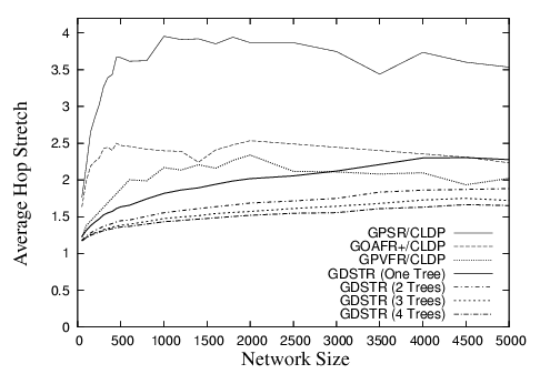
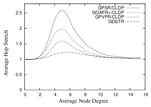
| Figure 6: Plot comparing the hop stretch for GDSTR to that for GPSR, GOAFR+ and GPVFR under CLDP planarization for unit radio networks in a 10 x 10 unit square. |
GDSTR has the best performance for most of the range: that is, GDSTR routes packets along shorter paths than the other algorithms, and is thus likely to deliver packets faster and with less consumption of radio resources. The only exception is that GPVFR's stretch is a few percent less than GDSTR for node degrees higher than 9.
The differences in the performance of the various algorithms are most pronounced in the critical region of node degrees between 4 and 6. The reason is that networks in this region tend to have large outer perimeters and the voids that are generated are often concave. Packets tend to end up in a local minima fairly often for these topologies and the routing algorithm has to resort to forwarding the packet along a face (for the face routing algorithms) or along a tree (for GDSTR).
GPSR performs the worst because it uses a deterministic right hand rule when forwarding a packet along a face. It turns out that topologies in the critical region typically present nodes that need to switch to face traversal with one good forwarding direction and one terrible alternative. By choosing the same direction consistently, GPSR gets it wrong about half the time.
GOAFR+ is better than GPSR because it uses an expanding ellipse to bound the search radius. GOAFR+ picks a random forwarding direction to start with, but instead of forwarding continuously along a face, GOAFR+ keeps track of how far it has gone along the face and if a packet seems to have wandered far enough along a face and not made any apparent progress toward the destination, GOAFR will make the packet backtrack. By expanding the area of the search incrementally, GOAFR ensures that the length of the final path traversed is no longer than a constant multiple of the optimal path.
GPVFR tries to pick the optimal forwarding direction when it switches from greedy forwarding to face traversal. It does so by maintaining several hops worth of information about its adjacent planar faces. It turns out that in practice, by maintaining information about nodes that are up to 4 hops away along the planar faces, GPVFR will often make the correct decision when the network density is low. When the network density is relatively high (above an average node degree of 9), CLDP produces planar faces that are relatively small (usually with fewer than seven points). Thus, under such circumstances, GPVFR has enough information to guarantee that it chooses the correct forwarding direction almost all the time, which explains why it performs better than GDSTR for node degrees higher than 9.
When two forwarding directions are available, GDSTR's tree-choosing heuristic of picking the tree with a root that is closest to the destination allows us to choose a good forwarding direction around a void most of the time. However, we believe that a more significant reason that explains why GDSTR outperforms the other algorithms in the critical region is that the convex hulls contain sufficient information to allow GDSTR to prune away many bad routing choices and route on a much reduced subtree that is often significantly smaller than large voids or the perimeter of the network (which often have one hundred or more nodes).
GDSTR can maintain multiple hull-trees. Figure 7 shows the effect of increasing the number of trees on the average hop stretch. Routing performance improves quite significantly when we increase the number of hull trees from one to two (achieving a peak improvement of approximately 10% in path and hop stretch); routing performance continues to improve with more trees but beyond two trees, the improvement is marginal. This is not surprising since two extremally-rooted trees are sufficient to approximate voids relatively well.
In Sections 5.1 and 5.2, we did not limit r, the maximum size for the convex hulls.
When we repeated the measurements for routing stretch for different values of r, we found that surprisingly, the value of r has a negligible effect on both path and hop stretch, i.e., the stretch for r was virtually indistinguishable from stretch when r is unlimited. We found that the reason for this is that although the hulls are bigger when r is limited and there are more intersections between the convex hulls of sibling nodes, intersections do not necessarily degrade routing performance as long as they are not particularly large or if they occur close to the leaves of a tree. In fact, intersections that do not contain any nodes do not affect routing performance.
It seems that even when r is reduced and the size of the hulls is increased, it is still relatively rare for nodes to fall into the intersections of hulls. Furthermore, intersections only matter when a packet is not forwarded in greedy mode. Since GDSTR forwards packets in greedy mode more than 75% of the time in our experimental setup and only occasionally switches to tree forwarding mode, it is not completely surprising that r does not seem to affect the aggregate routing performance.
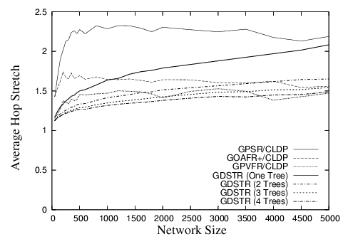
To understand how the routing performance of GDSTR scales with the size of the networks and also its performance on topologies that are not unit disk graphs (UDGs), we evaluated the routing performance of GDSTR on sets of networks with cross-shaped obstacles for sizes ranging from 50 to 5,000 nodes, while holding both node and obstacle densities constant. Without obstacles, the average node degrees of these networks would be 10; with the addition of obstacles, the average node degrees are reduced accordingly.
The hop stretch for networks with average node degrees approximately 6 and 7 are shown in Figures 8 and 9 respectively. These results are similar to that for random unit disk graphs with average node degrees 6 and 10 respectively [19].
Our results demonstrate that for sparse networks, the routing performance of GDSTR is consistently better than that for existing face routing algorithms, while for denser and larger networks, existing face routing algorithms can sometimes achieve slightly lower stretch. As mentioned, the reason is that extremally-rooted trees do not approximate voids quite as well when there are a large number of hops between the leaf nodes and the root.
In this section we present experimental results for the costs of GDSTR. Our main concern is with bandwidth since it is likely to be a limiting factor in radio networks. However we begin by discussing the storage costs of our system, since storage concerns were once a primary motivation for geographic routing algorithms.
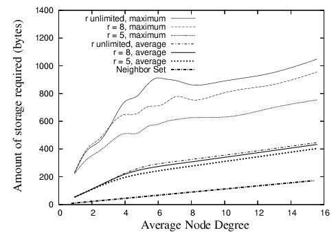
Figure 10 shows the average and maximal storage required by any nodes over the range of densities investigated. We assume that a set of coordinates and a node identifier are 8 and 12 bytes in size respectively. We can see from the figure that the maximum is about 1,000 bytes. This amount of storage is hardly a concern for modern sensor devices like the Mica2 [32], which has 128K of program memory and 512K of flash RAM.
The figure shows the storage requirements when GDSTR uses two hull trees. In general, GDSTR with two hull trees requires more than twice as much storage on average as existing face routing algorithms at low network densities. However, as the network density increases, the storage requirement of the neighbor set becomes comparable to the storage requirement for the hull trees.
The figure also shows the effect of limiting the size of the convex hulls, r, on storage. These results show that by limiting r, there is negligible effect on the average storage requirement. When r = 5, we can reduce the maximum storage required by up to 30% at low network densities. Since the associated storage costs are small, we find that there is no compelling reason for us to limit the size of the convex hulls in practice.
|
| Figure 10: Amount of routing state stored at each node for various values of r for GDSTR with two hull trees. |
In the following experiments that measure the costs of stabilization and maintenance, we compare the costs of GDSTR with the cost of building and maintaining a planar graph with CLDP. The reason is that the other associated costs of existing geographic face routing algorithms [12,16,20] are small relative to the cost of CLDP. The costs for GPSR [12] and GOAFR+ [16] are negligible; GPVFR [20] does impose some maintenance cost on the network to maintain its face information, but the cost is also small relative to CLDP.
We quantify the bandwidth costs for each algorithm in terms of the number of messages sent or forwarded by nodes during stabilization and repair. For GDSTR, we count the number of keepalive messages that contain new hull information. For CLDP, we count the probe messages.
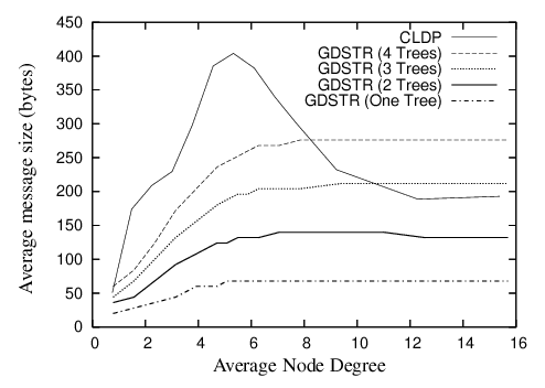
The average size of these messages is shown in Figure 11. As shown, the relative sizes of the CLDP probes and GDSTR broadcast messages are comparable. CLDP probes are largest in the critical region (average node degree 4 to 8) because the probes contain the points on the faces and these networks tend to have the largest perimeters.
Startup Costs. To investigate the startup costs for a network, we start all the nodes in the network at approximately the same time and measure the average number of messages sent by each node before the network converges.
CLDP involves a locking mechanism, so a configuration involving binary backoff will likely be able to optimize its startup performance. We do not know the optimal parameters, so we used the following simple probe model: all nodes have the same probing period with a 20% jitter (to avoid synchronization), and at the start of each period, a node probes all the links that require probing. If a reply is received, it is acted on immediately. If a probe message is dropped because it encounters a locked edge, the node will resend the probe during the next probe interval. A node is deemed to have converged when all its links are marked either dormant or non-routable and it does not have to initiate any more probes during the next probing interval. Similarly, a GDSTR node is deemed to have converged when it no longer needs to broadcast hull information in its keepalive messages.
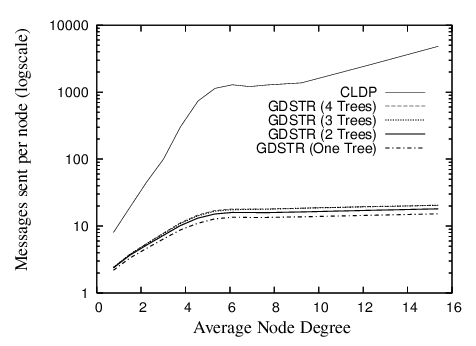
In Figure 12, we plot the average number of messages that each node in the network would have sent or forwarded before the network stabilizes, with all nodes starting up without any state. As shown, CLDP sends about two orders of magnitude more messages than GDSTR before the network stabilizes. For node degrees between 6 and 14, each CLDP node will send about 1,500 messages; for GDSTR, the corresponding number is slightly more than 10 messages.
There are two main reasons why CLDP imposes such a high overhead:
We see in Figure 12 that the startup costs for CLDP increases rapidly until node degree 6 and starts to taper off thereafter. This is because below node degree 6, the experimental topologies usually consist of several small disjoint networks. As the node degree increases, the networks become larger and more tree-like, and they tend to have larger perimeters that are costly to probe. After a critical density of about node degree 6, the networks become more connected, and their perimeters are somewhat more convex. The probing costs do not increase much at this stage with increasing density because the network perimeters either stay relatively constant or may even shrink slightly. The probing costs for CLDP are also proportional to the number of edges in the network graph however, so when the network density increases beyond node degree 8, the increase in the number of edges (links) becomes the dominating factor and we again see an increase in the CLDP probing cost.
Figure 12 also shows that the number of messages required per node by GDSTR plateaus at node degree 6 and increases only slightly thereafter. The reason for this is that the number of update messages that GDSTR requires is a function of the network diameter D. It turns out that since the nodes have unit radio range and are all contained within a 10 x 10 unit square, D is somewhat constant for densities higher than node degree 6.
Incremental Costs. To quantify the bandwidth required to update routing state when a new node joins and to repair routing state after a node fails, we measure the costs of adding and removing a single node from a stable network as follows: after a network has stabilized, we remove one node and count the number of messages sent per node. After the network has stabilized once again, we add the removed node back to the network and take the same measurement. We repeat this process on 20 randomly chosen nodes for each network and average the results to obtain the average cost per node change in each network.
In Figure 13, we plot the number of messages that are sent per node in order for the system to converge after one node join or departure. The peak for CLDP is about 200 messages per node at a node degree of 6. When a node joins the network for CLDP, new links are created between it and all its immediate neighbors and these new links are probed independently by the various nodes; when a node fails, its adjoining neighbors will probe all the adjacent links that are marked non-routable, in case there is the need to revive a non-routable link to restore connectivity. We see that the costs for node joins and departures are comparable, except for high network densities. The likely reason for this is that at high densities, node failures are significantly more costly than node joins because more links are re-probed for node failures and the number of such links is proportional to the node degree.
The join costs for GDSTR are uniformly low at approximately 3 messages per node; the repair costs after a node failure are highest in the region with node degree between 2 and 6 and falls gradually with increasing node density. The latter is because the likelihood of failure for an intermediate node is much higher at lower node densities (with a maximum of approximately 15 messages) and for high node densities, node failures are more likely to occur at the leaf nodes. Note that these figures are averaged over only the nodes that are affected by a node join or departure.
The bandwidth costs for updating a planar graph with CLDP incrementally are significantly lower than that for en masse stabilization at startup. In fact they can be interpreted also as the cost to stabilize for CLDP when the network grows one node at a time.
Discussion. We chose to evaluate startup and maintenance in terms of message count rather than convergence time because the system parameters for both CLDP and GDSTR can be tuned to achieve faster convergence. For example, the probing rate for CLDP can be increased and for GDSTR, nodes can broadcast update messages as and when there are changes in its hull trees instead of waiting to piggyback the information on keepalive messages. The total amount of information to be transmitted to bring the routing information to a consistent state is however the same in all cases. In fact, we can work out the fundamental limit on convergence time by dividing the volume of messages to be transmitted by the maximal achievable bandwidth of the radios.
In this section, we summarize what happens to cost as we scale up the network size to 5,000 nodes for the networks with cross-shaped obstacles.
Storage Costs. The average storage required per node is somewhat independent of network size and is about 300 bytes over the entire range of network topologies that we investigated; the maximal storage requirement increases steadily with network size, but it does not exceed 1,300 bytes even when the network size is scaled up to 5,000 nodes.
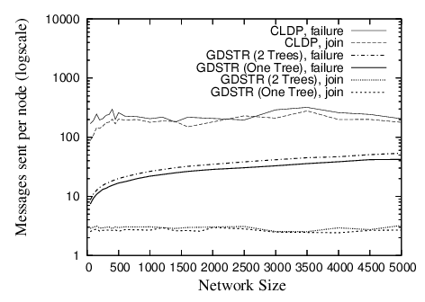
Bandwidth Costs. For large networks, the initial startup costs where all nodes start from a fresh state is not important, since large networks will have to be turned on incrementally. In Figure 14, we plot the average number of messages that are sent per node for CLDP and GDSTR for increasing network size for networks with mean node degree 7 and a constant obstacle density.
|
| Figure 14: Packets sent or forwarded per node when a new node joins or when an existing node fails for networks with cross-shaped obstacles and mean node degree 7. See Figure 9 for corresponding routing performance. |
The average number of messages sent per node for CLDP seems independent of the network size. For GDSTR, we see that messages sent per node for each incremental node join and network repair increase very gradually with network size. As before, node joins for GDSTR are relatively cheap, while repairs after network departures are slightly more costly. Individual node joins and network repairs only affect a fraction of the nodes in the network (typically less than 20% and decreasing with increasing network size).
The key insight of our work is that for geographic routing, it is no less efficient to use two hull trees instead of a planar graph as the backup routing topology when greedy forwarding fails, and it is significantly easier to build and maintain hull trees than a planar graph. Our simulations have demonstrated that GDSTR requires an order of magnitude less maintenance bandwidth than CLDP, while achieving lower path and hop stretch than existing geographic face routing algorithms.
GDSTR is immediately applicable to a large class of stationary wireless networks, e.g. roofnets [1,30] and sensornets [9,27]. While we have not explicitly evaluated the performance of GDSTR for mobile networks, our simulations show that GDSTR requires only a small number of packets to set up and repair its hull trees. This suggests that it is quite plausible that GDSTR will work well in a mobile setting with some tuning and optimization. It remains as future work to implement and evaluate GDSTR in a practical mobile environment.
While GDSTR is currently implemented over two-dimensional Cartesian coordinates, it is generalizable to coordinates in higher dimensional spaces, since convex hulls are generalizable to higher dimensions. An open question is whether GDSTR can achieve better routing stretch in higher dimensional space.
We thank the anonymous reviewers for their insightful comments and Dan Rubenstein for shepherding this paper. We also thank Eric Demaine, Young-Jin Kim, George Lee, Ji Li, Sayan Mitra, David Schultz, and Jijon Sit for their helpful comments on the early drafts of this paper.
[2] P. Bose, P. Morin, I. Stojmenovic, and J. Urrutia. Routing with guaranteed delivery in ad hoc wireless networks. Wireless Networks, 7(6):609-616, 2001.
[3] G. G. Finn. Routing and addressing problems in large metropolitan-scale internetworks. Technical Report ISI/RR-87-180, ISI, March 1987.
[4] R. Fonseca, S. Ratnasamy, J. Zhao, C. T. Ee, D. Culler, S. Shenker, and I. Stoica. Beacon Vector Routing: Scalable point-to-point routing in wireless sensornets. In Proceedings of NSDI 2005, pages 329-342, May 2005.
[5] K. Gabriel and R. Sokal. A new statistical approach to geographic variation analysis.Systematic Zoology, 18:259-278, 1969.
[6] R. Graham. An efficient algorithm for determining the convex hull of a finite planar set.Info. Proc. Letters, 1:132-133, 1972.
[7] T. Hou and V. Li. Transmission range control in multihop packet radio networks.IEEE Transactions on Communications, 34(1):38-44, 1986.
[8] D. B. Johnson and D. A. Maltz. Dynamic source routing in ad hoc wireless networks.In Mobile Computing, volume 353. 1996.
[9] J. M. Kahn, R. H. Katz, and K. S. J. Pister. Next century challenges: Mobile networking for ''smart dust''. In Proceedings of Mobicom '99, pages 271-278, August 1999.
[10] B. Karp. Geographic Routing for Wireless Networks. PhD thesis, 2000.
[11] B. Karp. Challenges in geographic routing: Sparse networks, obstacles, and traffic provisioning, May 2001.
[12] B. Karp and H. T. Kung. GPSR: greedy perimeter stateless routing for wireless networks. In Proceedings of Mobicom 2000, pages 243-254, Boston, MA, August 2000.
[13] Y.-J. Kim, R. Govindan, B. Karp, and S. Shenker. Geographic routing made practical. In Proceedings of NSDI 2005, pages 217-230, May 2005.
[14] Y.-J. Kim, R. Govindan, B. Karp, and S. Shenker. On the pitfalls of geographic face routing. In Proceedings of DIAL-M-POMC 2005, September 2005.
[15] E. Kranakis, H. Singh, and J. Urrutia. Compass routing on geometric networks. In Proceedings of the 11th Canadian Conference on Computational Geometry, pages 51-54, Vancouver, August 1999.
[16] F. Kuhn, R. Wattenhofer, Y. Zhang, and A. Zollinger. Geometric ad-hoc routing: Of theory and practice. In Proceedings of PODC 2003, pages 63-72, July 2003.
[17] F. Kuhn, R. Wattenhofer, and A. Zollinger. Worst-Case Optimal and Average-Case Efficient Geometric Ad-Hoc Routing. In Proceedings of MobiHoc 2003, pages 267-278, June 2003.
[18] B. Leong. Geographic routing network simulator, 2004. https://web.mit.edu/benleong/www/netsim.
[19] B. Leong. New Techniques for Geographic Routing. PhD thesis, 2006.
[20] B. Leong, S. Mitra, and B. Liskov. Path vector face routing: Geographic routing with local face information. In Proceedings of ICNP 2005, pages 147-158, November 2005.
[21] X. Li, Y. J. Kim, R. Govindan, and W. Hong. Multi-dimensional range queries in sensor networks. In Proceedings of SenSys 2003, pages 63-75, November 2003.
[22] J. Newsome and D. Song. GEM: Graph EMbedding for routing and data-centric storage in sensor networks without geographic information. In Proceedings of SenSys 2003, pages 76-88, November 2003.
[23] C. Perkins. Ad-hoc on-demand distance vector routing. In Proceedings of IEEE MILCOM '97, November 1997.
[24] C. Perkins and P. Bhagwat. Highly dynamic destination-sequenced distance-vector routing (DSDV) for mobile computers. In Proceedings of ACM SIGCOMM'94 Conference, pages 234-244, August 1994.
[25] S. Radhakrishnan, G. Racherla, C. N. Sekharan, N. S. V. Rao, and S. G. Batsell. DST - a routing protocol for ad hoc networks using distributed spanning trees. In IEEE Wireless Communications and Networking Conference, 1999.
[26] A. Rao, C. H. Papadimitriou, S. Shenker, and I. Stoica. Geographic routing without location information. In Proceedings of Mobicom 2003, pages 96-108, San Diego, CA, September 2003.
[27] S. Ratnasamy, B. Karp, S. Shenker, D. Estrin, R. Govindan, L. Yin, and F. Yu. Data-centric storage in sensornets with ght, a geographic hash table. Mobile Networks and Applications (MONET), Journal of Special Issues on Mobility of Systems, Users, Data, and Computing, 2003.
[28] S. Ratnasamy, B. Karp, L. Yin, F. Yu, D. Estrin, R. Govindan, and S. Shenker. GHT: A geographic hash table for data-centric storage in sensornets. In Proceedings of the First ACM International Workshop on Wireless Sensor Networks and Applications (WSNA), September 2002.
[29] K. Seada, A. Helmy, and R. Govindan. On the effect of localization errors on geographic face routing in sensor networks. In Proceedings of IPSN'04, pages 71-80, April 2004.
[30] T. J. Shepard. A channel access scheme for large dense packet radio networks. In Proceedings of the ACM SIGCOMM '96 Conference. ACM SIGCOMM, August 1996.
[31] H. Takagi and L. Kleinrock. Optimal transmission ranges for randomly distributed packet radio terminals. IEEE Transactions on Communications, 32(3):246-257, 1984.
[32] C. Technlogies. Mica2 series wireless measurement system. https://www.xbow.com.
[33] G. T. Toussaint. The relative neighbourhood graph of a finite planar set. Pattern Recognition, 12:261-268, 1980.
[34] G. Xing, C. Lu, R. Pless, and Q. Huang. On greedy geographic routing algorithms in sensing-covered networks. In Proceedings of MobiHoc '04, pages 31-42, May 2004.
[35] Y. Zhao, B. Li, Q. Zhang, Y. Chen, and W. Zhu. Hop ID based routing in mobile ad hoc networks. In Proceedings of ICNP 2005, pages 179-190, November 2005.
|
This paper was originally published in the Proceedings of the
3rd Symposium on Networked Systems Design and Implementation (NSDI '06) May 8–10, 2006, San Jose, CA Last changed: 3 May 2006 jel |