| ||||||||||||||||||||||||||||||||||||||||||||||||||||
|
NSDI '04 Paper
[NSDI '04 Technical Program]
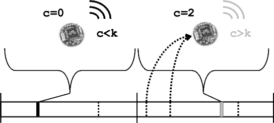
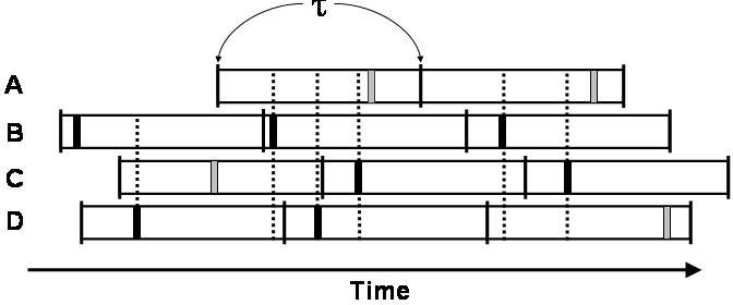
Trickle uses "polite gossip" to exchange code metadata with nearby network neighbors. It breaks time into intervals, and at a random point in each interval, it considers broadcasting its code metadata. If Trickle has already heard several other motes gossip the same metadata in this interval, it politely stays quiet: repeating what someone else has said is rude. When a mote hears that a neighbor is behind the times (it hears older metadata), it brings everyone nearby up to date by broadcasting the needed pieces of code. When a mote hears that it is behind the times, it repeats the latest news it knows of (its own metadata); following the first rule, this triggers motes with newer code to broadcast it. More formally, each mote maintains a counter c, a threshold k, and a timer t in the range [0,τ]. k is a small, fixed integer (e.g., 1 or 2) and τ is a time constant. We discuss the selection of τ in depth in Section 6. When a mote hears metadata identical to its own, it increments c. At timet, the mote broadcasts its metadata if c<k . When the interval of size τ completes, c is reset to zero and t is reset to a new random value in the range [0,τ]. If a mote with code φ hears a summary for φ-x, it broadcasts the code necessary to bring φ-x up to φ. If it hears a summary for φ+x, it broadcasts its own summary, triggering the mote with φ+x to send updates. Figure 3 has a visualization of Trickle in operation on a single mote for two intervals of length τ with a k of 1 and no new code. In the first interval, I₁, the mote does not hear any transmissions before its t, and broadcasts. In the second interval, I₂, it hears two broadcasts of metadata identical to its, and so suppresses its broadcast. Using the Trickle algorithm, each mote broadcasts a summary of its data at most once per period τ. If a mote hears k motes with the same program before it transmits, it suppresses its own transmission. In perfect network conditions - a lossless, single-hop topology - there will be k transmissions every τ. If there are n motes and m non-interfering single-hop networks, there will be km transmissions, which is independent of n. Instead of fixing the per-mote send rate, Trickle dynamically regulates its send rate to the network density to meet a communication rate, requiring no a priori assumptions on the topology. In each interval τ, the sum of receptions and sends of each mote is k.
The random selection of t uniformly distributes the
choice of who broadcasts in a given interval. This evenly
spreads the transmission energy load across the network. If
a mote with n neighbors needs an update, the expected
latency to discover this from the beginning of the interval
is This km transmission count depends on three assumptions: no packet loss, perfect interval synchronization, and a single-hop network. We visit and then relax each of these assumptions in turn. Discussing each assumption separately allows us to examine the effect of each, and in the case of interval synchronization, helps us make a slight modification to restore scalability.
| ||||||||||||||||||||||||||||||||||||||||||||||||||||||||||
 |
The above results assume that all motes have synchronized intervals. Inevitably, time synchronization imposes a communication, and therefore energy, overhead. While some networks can provide time synchronization to Trickle, others cannot. Therefore, Trickle should be able to work in the absence of this primitive.
Unfortunately, without synchronization, Trickle can suffer from the short-listen problem. Some subset of motes gossip soon after the beginning of their interval, listening for only a short time, before anyone else has a chance to speak up. If all of the intervals are synchronized, the first gossip will quiet everyone else. However, if not synchronized, it might be that a mote's interval begins just after the broadcast, and it too has chosen a short listening period. This results in redundant transmissions.
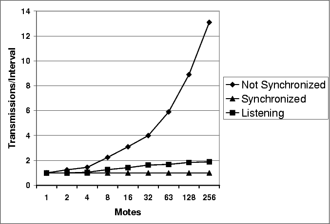 |
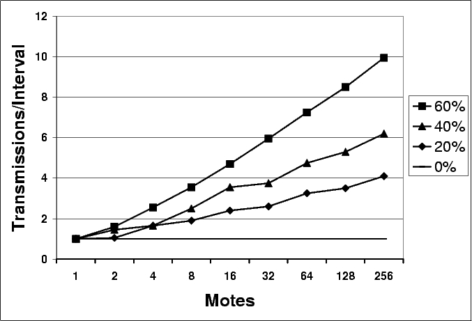
Figure 5 shows an instance of this phenomenon. In this example, mote B selects a small t on each of its three intervals. Although other motes transmit, mote B never hears those transmissions before its own, and its transmissions are never suppressed. Figure 6 shows how the short-listen problem effects the transmission rate in a lossless network with k=1. A perfectly synchronized single-hop network scales perfectly, with a constant number of transmissions. In a network without any synchronization between intervals, however, the number of transmissions per interval increases significantly.
The short-listen problem causes the number of transmissions to scale as O(√n) with network density. ² Unlike loss, where extra O(log(n)) transmissions are sent to keep the worst case mote up to date, the additional transmissions due to a lack of synchronization are completely redundant, and represent avoidable inefficiency.
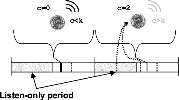
To remove the short-listen effect, we modified Trickle slightly. Instead of picking a t in the range [0,τ], t is selected in the range [0.5τ,τ], defining a ``listen-only'' period of the first half of an interval. Figure 7 depicts the modified algorithm. A listening period improves scalability by enforcing a simple constraint. If sending a message guarantees a silent period of some time T that is independent of density, then the send rate is bounded above (independent of the density). When a mote transmits, it suppresses all other motes for at least the length of the listening period. With a listen period of τ/2, it bounds the total sends in a lossless single-hop network to be 2k, and with loss scales as O(2k ⋅ log(n)), returning scalability to the O(log(n)) goal.
 |
The ``Listening'' line in Figure 6 shows the number of transmissions in a single-hop network with no synchronization when Trickle uses this listening period. As the network density increases, the number of transmissions per interval asymptotically approaches two. The listening period does not harm performance when the network is synchronized: there are k transmissions, but they are all in the second half of the interval.
To work properly, Trickle needs a source of randomness; this can come from either the selection of t or from a lack of synchronization. By using both sources, Trickle works in either circumstance, or any point between the two (e.g., partial or loose synchronization).
(a)Total Transmissions per Interval |
(b) Receptions per Transmission |
 (c) Redundancy |
|
| ||
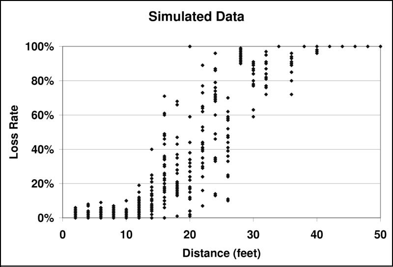
To understand Trickle's behavior in a multi-hop network, we used TOSSIM, randomly placing motes in a 50'x50' area with a uniform distribution, a τ of one second, and a k of 1. To discern the effect of packet collisions, we used both TOSSIM-bit and TOSSIM-packet (the former models collisions, and the latter does not). Drawing from the loss distributions in Figure 1, a 50'x50' grid is a few hops wide. Figure 8 shows the results of this experiment.
Figure 8(a) shows how the number of transmissions per interval scales as the number of motes increases. In the absence of collisions, Trickle scales as expected, at O(log(n)). This is also true in the more accurate TOSSIM-bit simulations for low to medium densities; however, once there is over 128 motes, the number of transmissions increases significantly.
This result is troubling - it suggests that Trickle cannot scale to very dense networks. However, this turns out to be a limitation of TinyOS's CSMA as network utilization increases, and not Trickle itself. Figure 8(b) shows the average number of receptions per transmission for the same experiments. Without packet collisions, as network density increases exponentially, so does the reception/transmission ratio. Packet collisions increase loss, and therefore the base of the logarithm in Trickle's O(log(n)) scalability. The increase is so great that Trickle's aggregate transmission count begins to scale linearly. As the number of transmissions over space increases, so does the probability that two will collide.
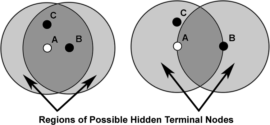 |
As the network becomes very dense, it succumbs to the hidden terminal problem, a known issue with CSMA protocols. In the classic hidden terminal situation, there are three nodes, A, B, and C, with effective carrier sense between A and B as well as A and C. However, as B and C do not hear one another, a CSMA protocol will let them transmit at the same time, colliding at A, who will hear neither. In this situation, B is a hidden terminal to C and vice versa. Figure 9 shows an instance of this phenomenon in a simplistic disk model.
In TOSSIM-bit, the reception/transmission ratio plateaus around seventy-five: each mote thinks it has about seventy-five one-hop network neighbors. At high densities, many packets are being lost due to collisions due to the hidden terminal problem. In the perfect scaling model, the number of transmissions for m isolated and independent single-hop networks is mk. In a network, there is a physical density (defined by the radio range), but the hidden terminal problem causes motes to lose packets; hearing less traffic, they are aware of a smaller observed density. Physical density represents the number of motes who can hear a transmission in the absence of any other traffic, while observed density is a function of other, possibly conflicting, traffic in the network. Increasing physical density also make collision more likely; observed density does not necessarily increase at the same rate.
When collisions make observed density lower than physical density, the set of motes observed to be neighbors is tied to physical proximity. The set of motes that can interfere with communication by the hidden terminal problem is larger when two motes are far away than when they are close. Figure 9 depicts this relationship.
Returning to Figure 8(b), from each mote's perspective in the 512 and 1024 mote experiments, the observed density is seventy-five neighbors. This does not change significantly as physical density increases. As a mote that can hear n neighbors, ignoring loss and other complexities, will broadcast in an interval with probability 1/n, the lack of increase in observed density increases the number of transmissions (e.g., (512/75) -> (1024/75)).
TOSSIM simulates the mica network stack, which can handle approximately forty packets a second. As utilization reaches a reasonable fraction of this (e.g., 10 packets/second, with 128 nodes), the probability of a collision becomes significant enough to affect Trickle's behavior. As long as Trickle's network utilization is low, it scales as expected. However, increased utilization affects connectivity patterns, so that Trickle must transmit more than in an quiet network. The circumstances of Figure 8, very dense networks and a tiny interval, represent a corner case. As we present in Section 5, maintenance intervals are more likely to be on the order of tens of minutes. At these interval sizes, network utilization will never grow large as long as k is small.
To better understand Trickle in multi-hop networks, we use
the metric of redundancy. Redundancy is the portion
of messages heard in an interval that were unnecessary
communication. Specifically, it is each mote's expected
value of  , where s is 1 if the mote
transmitted and 0 if not. A redundancy of 0 means Trickle
works perfectly; every mote communicates k times. For
example, a mote with ak of 2, that transmitted
(s=1), and then received twice (c=2), would
have a redundancy of 0.5 (
, where s is 1 if the mote
transmitted and 0 if not. A redundancy of 0 means Trickle
works perfectly; every mote communicates k times. For
example, a mote with ak of 2, that transmitted
(s=1), and then received twice (c=2), would
have a redundancy of 0.5 (
![]() ): it communicated
50% more than the optimum of k.
): it communicated
50% more than the optimum of k.
Redundancy can be computed for the single-hop experiments with uniform loss (Figures 4 and 6). For example, in a single-hop network with a uniform 20% loss rate and a k of 1, 3 transmissions/interval has a redundancy of 1.4=((3⋅0.8)-1) as the expectation is that each mote receives 2.4 packets, and three motes transmit.
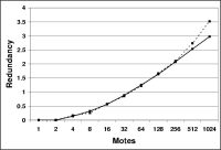
Figure 8(c) shows a plot of Trickle redundancy as network density increases. For a one-thousand mote- larger than any yet deployed - multi-hop network, in the presence of link asymmetry, variable packet loss, and the hidden terminal problem, the redundancy is just over 3.
Redundancy grows with a simple logarithm of the observed density, and is due to the simple problem outlined in Section 4.1: packets are lost. To maintain a communication rate for the worst case mote, the average case must communicate a little bit more. Although the communication increases, the actual per-mote transmission rate shrinks. Barring MAC failures, Trickle scales as hoped - O(log(n)) - in multi-hop networks.
 (a)Transmissions |
 (b)Receptions |
One of the goals of Trickle is to impose a low overhead. The above simulation results show that few packets are sent in a network. However, this raises the question of which motes sent those packets; 500 transmissions evenly distributed over 500 motes does not impose a high cost, but 500 messages by one mote does.
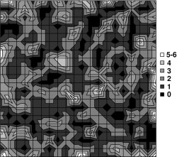
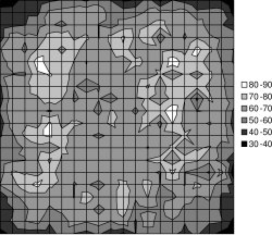
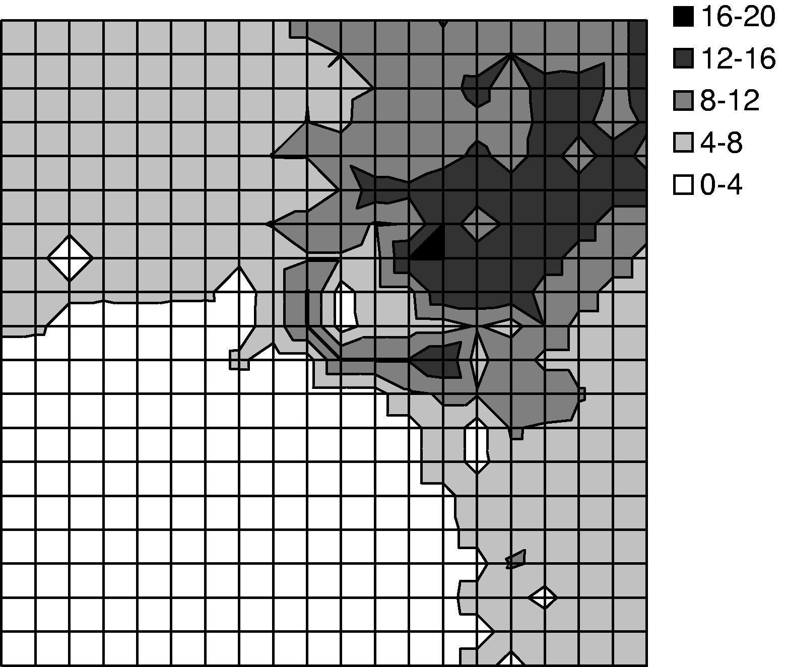
Figure 10(a) shows the transmission distribution for a simulated 400 mote network in a 20 mote by 20 mote grid with a 5 foot spacing (the entire grid was 95'x95'), run in TOSSIM-bit. Drawing from the empirical distributions in Figure 1, a five foot spacing forms a six hop network from grid corner to corner. This simulation was run with a τ of one minute, and ran for twenty minutes of virtual time. The topology shows that some motes send more than others, in a mostly random pattern. Given that the predominant range is one, two, or three packets, this non-uniformity is easily attributed to statistical variation. A few motes show markedly more transmissions, for example, six. This is the result of some motes being poor receivers. If many of their incoming links have high loss rates (drawn from the distribution in Figure 1), they will have a small observed density, as they receive few packets.
Figure 10(b) shows the reception distribution. Unlike the transmission distribution, this shows clear patterns. motes toward the edges and corners of the grid receive fewer packets than those in the center. This is due to the non-uniform network density; a mote at a corner has one quarter the neighbors as one in the center. Additionally, a mote in the center has many more neighbors that cannot hear one another; so that a transmission in one will not suppress a transmission in another. In contrast, almost all of the neighbors of a corner mote can hear one another. Although the transmission topology is quite noisy, the reception topography is smooth. The number of transmissions is very small compared to the number of receptions: the communication rate across the network is fairly uniform.
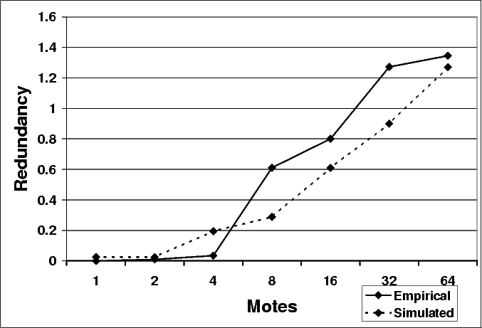
To evaluate Trickle's scalability in a real network, we
recreated, as best we could, the experiments shown in
Figures 6 and
8. We
placed motes on a small table, with their transmission
signal strength set very low, making the table a small
multi-hop network. With a ![]() of
one minute, we measured Trickle redundancy over a twenty
minute period for increasing numbers of
motes. Figure 11
shows the results. They show similar scaling to the results
from TOSSIM-bit. For example, the TOSSIM-bit results in
Figure 8(c)
show a 64 mote network having an redundancy of 1.1; the
empirical results show 1.35. The empirical results show that
maintenance scales as the simulation results indicate it
should: logarithmically.
of
one minute, we measured Trickle redundancy over a twenty
minute period for increasing numbers of
motes. Figure 11
shows the results. They show similar scaling to the results
from TOSSIM-bit. For example, the TOSSIM-bit results in
Figure 8(c)
show a 64 mote network having an redundancy of 1.1; the
empirical results show 1.35. The empirical results show that
maintenance scales as the simulation results indicate it
should: logarithmically.
The above results quantified the maintenance overhead. Evaluating propagation requires an implementation; among other things, there must be code to propagate. In the next section, we present an implementation of Trickle, evaluating it in simulation and empirically.
| Event | Action |
| τ Expires | Double τ up to τ-h. Reset c, pick a new t. |
| t Expires | If c<k, transmit. |
| Receive same metadata | Increment c. |
| Receive newer metadata | Set τ to τ-l. Reset c, pick a new t. |
| Receive newer code | Set τ to τ-l. Reset c, pick a new t. |
| Receive older metadata | Send updates. |
A large τ (gossiping interval) has a low communication overhead, but slowly propagates information. Conversely, a small τ has a higher communication overhead, but propagates more quickly. These two goals, rapid propagation and low overhead, are fundamentally at odds: the former requires communication to be frequent, while the latter requires it to be infrequent.
By dynamically scaling τ, Trickle can use its maintenance algorithm to rapidly propagate updates with a very small cost. τ has a lower bound, τ-l, and an upper bound τ-h. When τ expires, it doubles, up to τ-h. When a mote hears a summary with newer data than it has, it resets τ to be τ-l. When a mote hears a summary with older code than it has, it sends the code, to bring the other mote up to date. When a mote installs new code, it resets τ to τ-l, to make sure that it spreads quickly. This is necessary for when a mote receives code it did not request, that is, didn't reset its τ for. Figure 12 shows pseudocode for this complete version of Trickle.
Essentially, when there's nothing new to say, motes gossip infrequently: τ is set to τ-h. However, as soon as a mote hears something new, it gossips more frequently, so those who haven't heard it yet find out. The chatter then dies down, as τ grows from τ-l to τ-h.
By adjusting τ in this way, Trickle can get the best of
both worlds: rapid propagation, and low maintenance
overhead. The cost of a propagation event, in terms of
additional sends caused by shrinking τ, is approximately
![]() . For a τ-l of
one second and a &tau-h; of one hour, this is a cost of
eleven packets to obtain a three-thousand fold increase in
propagation rate (or, from the other perspective, a three
thousand fold decrease in maintenance overhead). The simple
Trickle policy, "every once in a while, transmit unless
you've heard a few other transmissions," can be used both to
inexpensively maintain code and quickly propagate it.
. For a τ-l of
one second and a &tau-h; of one hour, this is a cost of
eleven packets to obtain a three-thousand fold increase in
propagation rate (or, from the other perspective, a three
thousand fold decrease in maintenance overhead). The simple
Trickle policy, "every once in a while, transmit unless
you've heard a few other transmissions," can be used both to
inexpensively maintain code and quickly propagate it.
We evaluate an implementation of Trickle, incorporated into Maté, a tiny bytecode interpreter for TinyOS sensor networks [12]. We first present a brief overview of Maté and its Trickle implementation. Using TOSSIM, we evaluate how how rapidly Trickle can propagate an update through reasonably sized (i.e., 400 mote) networks of varying density. We then evaluate Trickle's propagation rate in a small (20 mote) real-world network.
Maté has a small, static set of code routines. Each routine can have many versions, but the runtime only keeps the most recent one. By replacing these routines, a user can update a network's program. Each routine fits in a single TinyOS packet and has a version number. The runtime installs routines with a newer version number when it receives them.
 (a) 5' Spacing, 6 hops |
 (b) 10' Spacing, 16 hops |
 (c) 15' Spacing, 32 hops |
 (d+) 20' Spacing, 40 hops |
Instead of sending entire routines, motes can broadcast version summaries. A version summary contains the version numbers of all of the routines currently installed. A mote determines that someone else needs an update by hearing that they have an older version.
Maté uses Trickle to periodically broadcast version summaries. In all experiments, code routines fit in a single TinyOS packet (30 bytes). The runtime registers routines with a propagation service, which then maintains all of the necessary timers and broadcasts, notifying the runtime when it installs new code. The actual code propagation mechanism is outside the scope of Trickle, but we describe it here for completeness. When a mote hears an older vector, it broadcasts the missing routines three times: one second, three seconds, and seven seconds after hearing the vector. If code transmission redundancy were a performance issue, it could also use Trickle's suppression mechanism. For the purpose of our experiments, however, it was not.
The Maté implementation maintains a 10Hz timer, which it uses to increment a counter. t and τ are represented in ticks of this 10Hz clock. Given that the current mote platforms can transmit on the order of 40 packets/second, we found this granularity of time to be sufficient. If the power consumption of maintaining a 10Hz clock were an issue (as it may be in some deployments), a non-periodic implementation could be used instead.
 |
 |
 |
 |
 |
 |
We used TOSSIM-bit to observe the behavior of Trickle during a propagation event. We ran a series of simulations, each of which had 400 motes regularly placed in a 20x20 grid, and varied the spacing between motes. By varying network density, we could examine how Trickle's propagation rate scales over different loss rates and physical densities. Density ranged from a five foot spacing between motes up to twenty feet (the networks were 95'x95' to 380'x380'). We set τ-l to one second and τ-h to one minute. From corner to corner, these topologies range from six to forty hops. ³
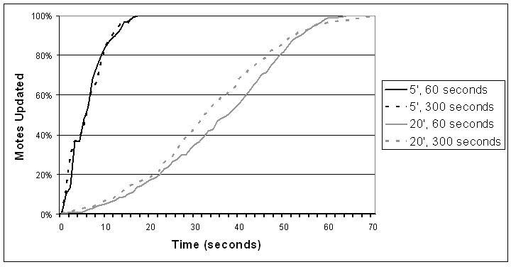
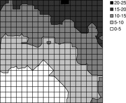
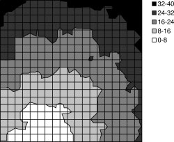
The simulations ran for five virtual minutes. motes booted with randomized times in the first minute, selected from a uniform distribution. After two minutes, a mote near one corner of the grid advertised a new Maté routine. We measured the propagation time (time for the last mote to install the new routine from the time it first appeared) as well as the topographical distribution of routine installation time. The results are shown in Figures 13 and 14. Time to complete propagation varied from 16 seconds in the densest network to about 70 seconds for the sparsest. Figure 13 shows curves for only the 5' and 20' grids; the 10' and 15' grid had similar curves.
Figure 14(a) shows a manifestation of the hidden terminal problem. This topography doesn't have the wave pattern we see in the experiments with sparser networks. Because the network was only a few hops in area, motes near the edges of the grid were able to receive and install the new capsule quickly, causing their subsequent transmissions to collide in the upper right corner. In contrast, the sparser networks exhibited a wave-like propagation because the sends mostly came from a single direction throughout the propagation event.
Figure 13 shows how adjusting τ-h changes the propagation time for the five and twenty foot spacings. Increasing τ-h from one minute to five does not significantly affect the propagation time; indeed, in the sparse case, it propagates faster until roughly the 95th percentile. This result indicates that there may be little trade-off between the maintenance overhead of Trickle and its effectiveness in the face of a propagation event.
A very large τ-h can increase the time to discover inconsistencies to be approximately τ-h/2. However, this is only true when two stable subnets (τ=τ-h) with different code reconnect. If new code is introduced, it immediately triggers motes to τ-l, bringing the network to action.
As Trickle was implemented as part of Maté, several other services run concurrently with it. The only one of possible importance is the ad-hoc routing protocol, which periodically sends out network beacons to estimate link qualities. However, as both Trickle packets and these beacons are very infrequent compared to channel capacity (e.g., at most 1 packet/second), this does not represent a significant source of noise.
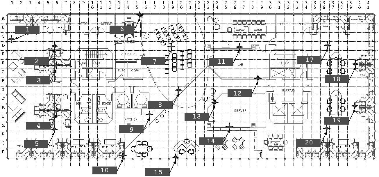
We deployed a nineteen mote network in an office area, approximately 160' by 40'. We instrumented fourteen of the motes with the TCP interface described in Section 2, for precise timestamping. When Maté installed a new piece of code, it sent out a UART packet; by opening sockets to all of the motes and timestamping when this packet is received, we can measure the propagation of code over a distributed area.
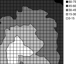
Figure 15 shows a picture of the office space and the placement of the motes. motes 4, 11, 17, 18 and 19 were not instrumented; motes 1, 2, 3, 5, 6, 7, 8, 9, 10, 12, 13, 14, 15, and 20 were. mote 16 did not exist.
As with the above experiments, Trickle was configured with a τ-l of one second and a τ-h of one minute. The experiments began with the injection of a new piece of code through a TinyOS GenericBase, which is a simple bridge between a PC and a TinyOS network. The GenericBase broadcast the new piece of code three times in quick succession. We then logged when each mote had received the code update, and calculated the time between the first transmission and installation.
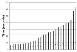
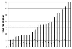
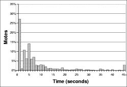
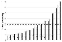
The left hand column of Figure 16 shows the results of these experiments. Each bar is a separate experiment (40 in all). The worst-case reprogramming time for the instrumentation points was just over a minute; the best case was about seven seconds. The average, shown by the dark dotted line, was just over twenty-two seconds for a τ-h of sixty seconds (Figure 16(a)), while it was thirty-two seconds for a τ-h of twenty minutes (Figure 16(b)).
The right hand column of Figure 16 shows a distribution of the time to reprogramming for individual motes across all the experiments. This shows that almost all motes are reprogrammed in the first ten seconds: the longer times in Figure 16 are from the very long tail on this distribution. The high loss characteristics of the mote radio, combined with t's exponential scaling, make this an issue. When scaling involves sending only a handful (e.g., log₂(60)) of packets in a neighborhood in order to conserve energy, long tails are inevitable.
In Figure 16, very few motes reprogram between one and two seconds after code is introduced. This is an artifact of the granularity of the timers used, the capsule propagation timing, and the listening period. Essentially, from the first broadcast, three timers expire: [τ-l/2,τ-l] for motes with the new code, [τ-l/2,τ-l] for motes saying they have old code, then one second before the first capsule is sent. This is approximately τ-l +1; with a τ-l of one second, this latency is two seconds.
The Maté implementation of Trickle requires few system resources. It requires approximately seventy bytes of RAM; half of this is a message buffer for transmissions, a quarter is pointers to the Maté routines. Trickle itself requires only eleven bytes for its counters; the remaining RAM is used by coordinating state such as pending and initialization flags. The executable code is 2.5 KB; TinyOS's inlining and optimizations can reduce this by roughly 30%, to 1.8K. The algorithm requires few CPU cycles, and can operate at a very low duty cycle.
Trickle draws on two major areas of prior research. Both assume network characteristics distinct from low-power wireless sensor networks, such as cheap communication, end-to-end transport, and limited (but existing) loss. The first area is controlled, density-aware flooding algorithms for wireless and multicast networks [6,15,18]. The second is epidemic and gossiping algorithms for maintaining data consistency in distributed systems [2,4,5].
Prior work in network broadcasts has dealt with a different problem than the one Trickle tackles: delivering a piece of data to as many nodes as possible within a certain time period. Early work showed that in wireless networks, simple broadcast retransmission could easily lead to the broadcast storm problem [18], where competing broadcasts saturate the network. This observation led to work in probabilistic broadcasts [15,20], and adaptive dissemination [9]. Just as with earlier work in bimodal epidemic algorithms [1], all of these algorithms approach the problem of making a best-effort attempt to send a message to all nodes in a network, then eventually stop.
For example, Ni et al. propose a counter-based algorithm to prevent the broadcast storm problem by suppressing retransmissions [18]. This algorithm operates on a single interval, instead of continuously. As results in Figure 16> show, the loss rates in the class of wireless sensor network we study preclude a single interval from being sufficient. Additionally, their studies were on lossless, disk-based network topologies; it is unclear how they would perform in the sort of connectivity observed in the real world [11].
This is insufficient for sensor network code propagation. For example, it is unclear what happens if a mote rejoins three days after the broadcast. For configurations or code, the new mote should be brought up to date. Using prior wireless broadcast techniques, the only way to do so is periodically rebroadcast to the entire network. This imposes a significant cost on the entire network. In contrast, Trickle locally distributes data where needed.
The problem of propagating data updates through a distributed system has similar goals to Trickle, but prior work has been based on traditional wired network models. Demers et al. proposed the idea of using epidemic algorithms for managing replicated databases [5], while the PlanetP project [4] uses epidemic gossiping for a a distributed peer-to-peer index. Our techniques and mechanisms draw from these efforts. However, while traditional gossiping protocols use unicast links to a random member of a neighbor set, or based on a routing overlay [2], Trickle uses only a local wireless broadcast, and its mechanisms are predominantly designed to address the complexities that result.
Gossiping through the exchange of metadata is reminiscent of SPIN's three-way handshaking protocol [9]; the Impala system, deployed in ZebraNet, uses a similar approach [14]. Specifically, Trickle is similar to SPIN-RL, which works in broadcast environments and provides reliability in lossy networks. Trickle differs from and builds on SPIN in three major ways. First, the SPIN protocols are designed for transmitting when they detect an update is needed; Trickle's purpose is to perform that detection. Second, the SPIN work points out that periodically re-advertising data can improve reliability, but does not suggest a policy for doing so; Trickle is such a policy. Finally, the SPIN family, although connectionless, is session oriented. When a node A hears an advertisement from node B, it then requests the data from node B. In contrast, Trickle never considers addresses. Taking the previous example, with Trickle B sends an implicit request, which a node besides A may respond to.
Trickle's suppression mechanism is inspired by the request/repair algorithm used in Scalable and Reliable Multicast (SRM) [6]. However, SRM focuses on reliable delivery of data through a multicast group in a wired IP network. Using IP multicast as a primitive, SRM has a fully connected network where latency is a concern. Trickle adapts SRM's suppression mechanisms to the domain of multi-hop wireless sensor networks.
Although both techniques - broadcasts and epidemics - have assumptions that make them inappropriate to problem of code propagation and maintenance in sensor networks, they are powerful techniques that we draw from. An effective algorithm must adjust to local network density as controlled floods do, but continually maintain consistency in a manner similar to epidemic algorithms. Taking advantage of the broadcast nature of the medium, a sensor network can use SRM-like duplicate suppression to conserve precious transmission energy and scale to dense networks.
In the sensor network space, Reijers et al. propose energy efficient code distribution by only distributing changes to currently running code [19]. The work focuses on developing an efficient technique to compute and update changes to a code image through memory manipulation, but does not address the question of how to distribute the code updates in a network or how to validate that nodes have the right code. It is a program encoding that Trickle or a Trickle-like protocol can use to transmit updates.
The TinyDB sensor network query system uses an epidemic style of code forwarding [16]. However, it depends on periodic data collection with embedded metadata. Every tuple routed through the network has a query ID associated with it and a mote requests a new query when it hears it. In this case, the metadata has no cost, as it would be sent anyways. Also, this approach does not handle event-driven queries for rare events well; the query propagates when the event occurs, which may be too late.
Using listen periods and dynamic τ values, Trickle meets the requirements set out in Section 1. It can quickly propagate new code into a network, while imposing a very small overhead. It does so using a very simple mechanism, and requires very little state. Scaling logarithmically with density, it can be used effectively in a wide range of networks. In one of our empirical experiments, Trickle imposes an overhead of less than three packets per hour, but reprograms the entire network in thirty seconds, with no effort from an end user.
A trade-off emerges between energy overhead and reprogramming rate. By using a dynamic communication rate, Trickle achieves a reprogramming rate comparable to frequent transmissions while keeping overhead comparable to infrequent transmissions. However, as Figure 16 shows, the exact relationship between constants such as τ-h and k is unclear in the context of these high loss networks. τ-l affects the head of the distribution , while τ-h affects the tail.
In this study, we have largely ignored the actual policy used to propagate code once Trickle detects the need to do so: Maté merely broadcasts code routines three times. Trickle suppression techniques can also be used to control the rate of code transmission. In the current Maté implementation, the blind code broadcast is a form of localized flood; Trickle acts as a flood control protocol. This behavior is almost the inverse of protocols such as SPIN [9], which transmits metadata freely but controls data transmission.
Assuming complete network propagation allows Trickle to decouple code advertisement from code transmission. As the protocol does not consider network addresses, the mote that advertises code - leading to an implicit request - may not be the one that transmits it. Instead of trying to enforce suppression on an abstraction of a logical group, which can become difficult in multi-hop networks, Trickle suppresses in terms of space, implicitly defining a group. Correspondingly, Trickle does not impose the overhead of discovering and maintaining logical groups, which can be significant.
One limitation of Trickle is that it currently assumes motes are always on. To conserve energy, long-term mote deployments often have very low duty cycles (e.g., 1%). Correspondingly, motes are rarely awake, and rarely able to receive messages. Communication scheduling schemes can define times for code communication, during which motes in the network wake up to run Trickle. Essentially, the Trickle time intervals become logical time, spread over all of the periods motes are actually awake. Understandably, this might require alternative tunings of τ-h and k. Trickle's scalability, however, stems from randomization and idle listening. As Section 8 showed, Trickle's transmission scalability suffers under a CSMA protocol as utilization increases. Another, and perhaps more promising, option is to use low power listening, where transmitters send very long start symbols so receivers can detect packets when sampling the channel at a very low rate [10]. For more dense networks, the receiver energy savings could make up for the transmitter energy cost.
Trickle was designed as a code propagation mechanism over an entire network, but it has greater applicability, and could be used to disseminate any sort of data. Additionally, one could change propagation scope by adding predicates to summaries, limiting the set of motes that consider them. For example, by adding a ``hop count'' predicate to local routing data, summaries of a mote's routing state could reach only two-hop network neighbors of the summary owner; this could be used to propagate copies of mote-specific information.
As sensor networks move from research to deployment, from laboratory to the real world, issues of management and reconfiguration will grow in importance. We have identified what we believe to be a core networking primitive in these systems, update distribution, and designed a scalable, lightweight algorithm to provide it.
 .
For time t,
.
For time t,  will have started
their intervals. From this, we can compute the expected time
after a transmission that another transmission will
occur. This is when
will have started
their intervals. From this, we can compute the expected time
after a transmission that another transmission will
occur. This is when

which is when  , that is, when
  time has passed. There
will therefore be O(√n)transmissions.
time has passed. There
will therefore be O(√n)transmissions.
|
This paper was originally published in the
Proceedings of the First Symposium on Networked Systems Design and Implementation,
March 29–31, 2004, San Francisco, CA, USA Last changed: 18 March 2004 ch |
|