|
MobiSys '03 Paper
[MobiSys '03 Tech Program Index]
| Pp. 113-128 of the Proceedings |  |
\Large Predictive Resource Management for Wearable Computing
Predictive Resource Management for Wearable Computing
Dushyanth Narayananf and M. Satyanarayananff
fCarnegie Mellon University and
fIntel Research Pittsburgh
{bumba,satya}@cs.cmu.edu
Abstract
Achieving crisp interactive response in resource-intensive
applications such as augmented reality, language translation, and
speech recognition is a major challenge on resource-poor wearable
hardware. In this paper we describe a solution based on
multi-fidelity computation supported by predictive resource
management. We show that such an approach can substantially reduce
both the mean and the variance of response time. On a benchmark
representative of augmented reality, we demonstrate a 60% reduction
in mean latency and a 30% reduction in the coefficient of
variation. We also show that a history-based approach to demand
prediction is the key to this performance improvement: by applying
simple machine learning techniques to logs of measured resource
demand, we are able to accurately model resource demand as a function
of fidelity.
1 Introduction
Resource-intensive applications such as speech recognition, language
translation, and augmented reality pose a dilemma for wearable
computing. Such applications are valuable because they support
hands-free interaction. However, their peak resource demands can
overwhelm the processing speed, memory, and battery capacity of
wearable hardware whose weight, size and form factor are limited by
user comfort. The result is sluggish interactive response that can
seriously distract a mobile user engaged in a physically and
cognitively demanding task such as bridge inspection, aircraft
maintenance or military action.
Technology improvements through Moore's Law will not solve this
problem. Rather, it is likely to persist because market forces
in wearable computing demand continuous improvements in user
comfort rather than just improvements in compute power. This
tension leads to the question addressed by this paper: How
can we achieve crisp interactive response for resource-intensive
applications on wearable computers?
In this paper, we show how multi-fidelity computation can help
to bound interactive latency by dynamically trading resource demand
for output quality, or fidelity. We describe the design,
implementation and evaluation of a system that supports multi-fidelity
computation. The system automatically makes runtime fidelity decisions
on the applications' behalf, thus freeing programmers from this
burden. To make sound fidelity decisions, it exploits
history-based prediction of application resource usage.
Our implementation is based on Odyssey [15,30], which
originally supported the concept of fidelity for stored data. This
work extends that concept to the broader notion of computational
fidelity and demonstrates its applicability to a new class of
applications. In the rest of this paper, the term "fidelity" will
mean "computational fidelity" and "Odyssey" will refer to the
multi-fidelity support added by us to the base system.
We have experimentally validated our approach using four
applications. Because of space limitations, we only describe one
application case study in detail here, and summarize the results of
the other three. Full details of the latter can be found in
Narayanan's dissertation [27]. Our key results can be
summarized as follows:
- Predictive resource management can bound response latency and
reduce its variability.
- History-based prediction of resource demand is feasible,
accurate, and necessary for this improvement.
- Legacy applications can be ported at modest
cost to a multi-fidelity programming model.
Section 2 describes our high-level design principles
and rationale. Section 3 describes our prototype API
for multi-fidelity computation, and the implementation of the runtime
support layer. It also explains our methodology for constructing
application-specific resource demand predictors, and describes one
example in detail. Section 4 presents a
comprehensive evaluation of the system: we measure the accuracy of
history-based prediction, the performance benefits of predictive
resource management, and the programming costs and runtime
overheads. Section 5 describes related work, and
Section 6 concludes with some directions for future
research.
2 Design rationale
2.1 Alternatives
There are three fundamentally different approaches to coping with
situations where application resource demand exceeds supply. One
approach is to prevent such situations by using QoS-based
resource reservations [22,26]. For example, an
application may be able to reserve a minimum fraction of a CPU and
thus guard against insufficient supply of this resource due to
competition from concurrent applications. As another example, it may
be possible to reserve bandwidth in a carefully controlled networking
environment. Unfortunately, enforcement of QoS-based reservations
requires operating system support that is rarely present in standard
OS distributions. More importantly, this approach fails when the peak
resource demand of a single application exceeds the capabilities of
the hardware it is running on.
The second approach is to acquire additional resources through
remote execution. Even a resource-impoverished wearable computer
such as the IBM Linux wristwatch [29] can use
compute servers to run resource-intensive applications. In previous
work, we described Spectra [14], a remote execution
subsystem layered on the multi-fidelity framework described here. We
are further exploring remote execution in current work [4].
However, there are many situations in which a mobile user has no
access to compute servers and must therefore rely solely on the
resources of his wearable computer. A different approach must be used
to handle those situations.
The third approach is to reduce resource demand through multi-fidelity
computation. As its name implies, multi-fidelity computation assumes
that an application is capable of presenting results at different
fidelities. Users prefer results of higher fidelity, but can tolerate
results of lower fidelity. A high-fidelity result requires greater
resources to compute than a low-fidelity result. When resources are
plentiful, the application generates high-fidelity results; when
resources are scarce, it generates low-fidelity results. By
dynamically varying fidelity, timely results can be generated over a
wide range of resource levels. We elaborate on this in the next
section.
2.2 Multi-fidelity computation
The classic notion of an algorithm has a fixed output specification
but variable resource demand. In contrast, it is the output
specification that is variable in a multi-fidelity
computation [32]. By setting runtime parameters called
fidelity metrics, we can obtain different outputs for the same
input. One can say, in effect, "Give me the best result you can
using no more than X units of resource R." R is typically
response latency in an interactive application, but it can also refer
to memory, energy, bandwidth or any other resource. Thus
multi-fidelity computations are a generalization of any-dimension
algorithms [25]. The latter can be viewed as
multi-fidelity computations which incrementally refine their output,
allowing them to be interrupted at any point to yield a result.
Multi-fidelity computation allows us to choose the best runtime
tradeoff between output quality and performance. In an interactive
application, each interactive operation can be viewed as a
multi-fidelity computation. At the beginning of each operation, its
fidelity metrics can be set to yield the desired response latency at
the current resource availability.
2.3 Motivating example
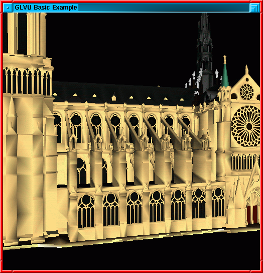 High fidelity (1.0)
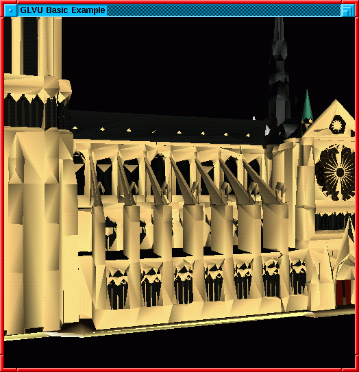 Low fidelity (0.1)
Figure 1: Effect of fidelity on 3-D rendering
Throughout this paper we will use augmented reality
(AR) [3] as the driving example to illustrate various
aspects of our system. Although AR is a relatively young technology,
it has already proved useful in a number of domains such as tourist
guides [12], power plant maintenance [11],
architectural design [37], and computer-supported
collaboration [5].
In AR, a user looks through a transparent heads-up display connected
to a wearable computer. Any displayed image appears to be
superimposed on the real-world scene before the user. AR thus creates
the illusion that the real world is visually merged with a virtual
world. This requires a precise correspondence between the two worlds.
As a user's orientation and location change, the displayed image must
rapidly and accurately track those changes. Sluggish tracking can be
distracting to the user and, in extreme cases, can result in symptoms
similar to sea-sickness.
3-D rendering, a computationally intensive operation, lies at
the heart of AR. Even a brief turn of the head by a user can result
in a complex scene having to be re-rendered multiple times. For
example, an architect might use AR for on-site design. This would
allow her to visualize the impact of proposed design changes such as
new windows or color schemes. Before converging on a final design, she
may iteratively try out many alternatives, viewing them from different
angles and under different hypothetical lighting conditions such as
moonlight or sunset.
3-D rendering for AR embodies many of the characteristics that
motivate the work described in this paper. First, it is extremely
resource intensive, particularly of CPU and memory. Second, to be
fully effective it must run on a lightweight wearable computer.
Third, crisp interactive response is critical. Fourth, there is a
fidelity metric, the resolution of the displayed image, that directly
impacts resource consumption.
Figure 1 illustrates the last point. The
high-fidelity figure on the left contains ten times as many polygons
as the low-fidelity figure on the right. Since CPU demand increases
with the number of polygons, the low-fidelity figure can be rendered
much faster. In many situations, the low-fidelity figure may be
acceptable; the user can always explicitly ask for re-rendering at
higher fidelity.
Low fidelity (0.1)
Figure 1: Effect of fidelity on 3-D rendering
Throughout this paper we will use augmented reality
(AR) [3] as the driving example to illustrate various
aspects of our system. Although AR is a relatively young technology,
it has already proved useful in a number of domains such as tourist
guides [12], power plant maintenance [11],
architectural design [37], and computer-supported
collaboration [5].
In AR, a user looks through a transparent heads-up display connected
to a wearable computer. Any displayed image appears to be
superimposed on the real-world scene before the user. AR thus creates
the illusion that the real world is visually merged with a virtual
world. This requires a precise correspondence between the two worlds.
As a user's orientation and location change, the displayed image must
rapidly and accurately track those changes. Sluggish tracking can be
distracting to the user and, in extreme cases, can result in symptoms
similar to sea-sickness.
3-D rendering, a computationally intensive operation, lies at
the heart of AR. Even a brief turn of the head by a user can result
in a complex scene having to be re-rendered multiple times. For
example, an architect might use AR for on-site design. This would
allow her to visualize the impact of proposed design changes such as
new windows or color schemes. Before converging on a final design, she
may iteratively try out many alternatives, viewing them from different
angles and under different hypothetical lighting conditions such as
moonlight or sunset.
3-D rendering for AR embodies many of the characteristics that
motivate the work described in this paper. First, it is extremely
resource intensive, particularly of CPU and memory. Second, to be
fully effective it must run on a lightweight wearable computer.
Third, crisp interactive response is critical. Fourth, there is a
fidelity metric, the resolution of the displayed image, that directly
impacts resource consumption.
Figure 1 illustrates the last point. The
high-fidelity figure on the left contains ten times as many polygons
as the low-fidelity figure on the right. Since CPU demand increases
with the number of polygons, the low-fidelity figure can be rendered
much faster. In many situations, the low-fidelity figure may be
acceptable; the user can always explicitly ask for re-rendering at
higher fidelity.
2.4 Predictive resource management
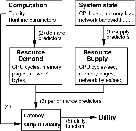 Figure 2: Mapping fidelity to utility
Before executing an interactive operation, an application must
determine its fidelity settings. Odyssey serves as an oracle in
making this decision. Its recommendation is based on a search of the
space of fidelity settings. This search requires Odyssey to predict
resource supply during the operation, as well as resource demand and
operation latency for different settings. It also requires Odyssey to
correctly reflect the user's current preferences in the tradeoff
between output quality and operation latency.
As Figure 2 shows, the complete prediction process can be
decomposed into five predictive mappings. Three of the mappings
relate to predicting operation latency:
(1) from system load statistics to resource supply;
(2) from fidelity to resource demand; and, (3)
from resource supply and demand to operation latency.
The other two mappings translate fidelity and latency predictions into
predictions of user satisfaction or utility:
(4) from fidelity to output quality; and, (5) from latency and output
quality to utility.
Odyssey performs mapping 1 using supply predictors that
monitor kernel load statistics through standard interfaces, and make
inferences based on gray-box knowledge [2] of
kernel resource management policies. It uses history-based demand
predictors to perform mapping 2, and performance predictors based on
a resource model for mapping 3. These components are described in
Sections 3.3 and 3.4.
Mapping 4 specifies the output quality we can expect at each setting
of each fidelity "knob". In general, this mapping would be
determined through studies of user perception. In this work, we make
the simplifying assumption that fidelity and output quality are
synonymous; in other words, that the mapping is trivial.
For example, we use the "JPEG level" parameter of a JPEG compression
algorithm as a measure of the output image quality; the work by
Chandra and Ellis [6] confirms that this is acceptable.
Mapping (5) is a utility function that captures current user
preferences. In a deployed system, utility functions would be
generated automatically from a GUI or by inferring user intent. In our
experimental prototype, we use the hand-crafted utility functions
described in Section 3.5.
Figure 2: Mapping fidelity to utility
Before executing an interactive operation, an application must
determine its fidelity settings. Odyssey serves as an oracle in
making this decision. Its recommendation is based on a search of the
space of fidelity settings. This search requires Odyssey to predict
resource supply during the operation, as well as resource demand and
operation latency for different settings. It also requires Odyssey to
correctly reflect the user's current preferences in the tradeoff
between output quality and operation latency.
As Figure 2 shows, the complete prediction process can be
decomposed into five predictive mappings. Three of the mappings
relate to predicting operation latency:
(1) from system load statistics to resource supply;
(2) from fidelity to resource demand; and, (3)
from resource supply and demand to operation latency.
The other two mappings translate fidelity and latency predictions into
predictions of user satisfaction or utility:
(4) from fidelity to output quality; and, (5) from latency and output
quality to utility.
Odyssey performs mapping 1 using supply predictors that
monitor kernel load statistics through standard interfaces, and make
inferences based on gray-box knowledge [2] of
kernel resource management policies. It uses history-based demand
predictors to perform mapping 2, and performance predictors based on
a resource model for mapping 3. These components are described in
Sections 3.3 and 3.4.
Mapping 4 specifies the output quality we can expect at each setting
of each fidelity "knob". In general, this mapping would be
determined through studies of user perception. In this work, we make
the simplifying assumption that fidelity and output quality are
synonymous; in other words, that the mapping is trivial.
For example, we use the "JPEG level" parameter of a JPEG compression
algorithm as a measure of the output image quality; the work by
Chandra and Ellis [6] confirms that this is acceptable.
Mapping (5) is a utility function that captures current user
preferences. In a deployed system, utility functions would be
generated automatically from a GUI or by inferring user intent. In our
experimental prototype, we use the hand-crafted utility functions
described in Section 3.5.
3 Interface and implementation
3.1 Programming interface
The multi-fidelity programming model is based on the notion of an
operation. An operation is the smallest user-visible unit of
execution, from user request to system response. Each operation
corresponds to one multi-fidelity computation, with fidelity metrics
settable at operation start. Examples include rendering an augmented
reality scene; recognizing a speech utterance and displaying the
recognized text; fetching and displaying a web image.
int register_fidelity(IN char *conf_file,
OUT int *optype_idp);
int begin_fidelity_op(IN const char *dataname,
IN int optype_id,
IN int num_params,
IN fid_param_val_t *params,
IN int num_fidelities,
OUT fid_param_val_t *fidelities,
OUT int *opidp);
int end_fidelity_op(IN int optype_id,
IN int opid,
IN failure_code failed);
| | C function prototypes for the API described in Section 3.1.
|
| |
Figure 3: The Odyssey multi-fidelity API
description glvu:render
logfile /usr/odyssey/etc/glvu.render.log
constraint latency 1.0
param polygons ordered 0-infinity
fidelity resolution ordered 0.01-1
hintfile /usr/odyssey/lib/glvu_hints.so
hint cpu glvu_render_cpu_hint
update glvu_render_update
utility glvu_render_utility
| | The first five lines specify a descriptive tag for the operation;
a pathname for writing log data; a target latency for the operation;
a non-tunable parameter; and a fidelity metric. The last four lines
specify a binary hint module and name its entry points.
|
| |
Figure 4: Application Configuration File for rendering
Figure 3 shows the basic multi-fidelity
API. register_fidelity is called at application startup. Odyssey
then reads an Application Configuration File (ACF), which specifies
the multi-fidelity operation type, its fidelity metrics, and their
value ranges (Figure 4).
The ACF also specifies nontunable parameters: runtime variables
such as input data size that affect resource demand, but are not
adaptable. For example, the resource demand of rendering depends not
only on the resolution, but also on the polygon count of the original,
full-resolution scene.
Finally, the ACF specifies an application-specific hint
module. This binary module contains the application-specific resource
demand predictors and the user utility function. For efficient runtime
invocation of the demand predictors and utility function, the hint
module is loaded into Odyssey's address space. We are looking at ways
to retain the efficiency, but improve on the safety, of this approach.
Before each operation, the application invokes begin_fidelity_op,
and passes in the nontunable parameters. Odyssey computes and returns
the optimal fidelity value(s) for the operation. After each
operation, the application calls end_fidelity_op. Odyssey then
logs the operation's measured resource demand: these logs are used for
history-based resource demand prediction
(Section 3.4).
3.2 System architecture
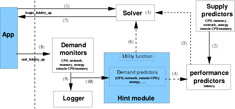
| Shaded boxes represent application-specific components; components to
the right of the dotted line are part of Odyssey. The arrows show the
data flow between components; dashed arrows correspond to interactions
that occur many times for a single invocation of the API. The numbers
correspond to the steps in Section 3.2.
|
Figure 5: System support for the multi-fidelity API
Odyssey is implemented as a user-level process on a standard Linux 2.4
kernel. Its primary functionality - making fidelity decisions - is
triggered by begin_fidelity_op and implemented in the following
steps, numbered as in Figure 5:
- The application passes in the nontunable parameters.
- Supply predictors estimate the application's resource
supply for the near future (mapping 1 of Figure 2).
- An iterative solver searches the fidelity space for the best
candidate.
- Demand predictors map fidelity to resource demand (mapping 2).
- A performance predictor estimates latency given
supply and demand predictions (mapping 3).
- A utility function evaluates the proposed
fidelity-performance tradeoff (mapping 5).
- After several iterations of steps 0-0,
the solver returns the fidelity with the highest utility.
The system's second function - monitoring and logging - is
triggered by end_fidelity_op:
- Demand monitors measure the resources consumed by the
just-concluded operation.
- A logger records the resource demand, fidelity, and nontunable
parameter values to a disk file.
- These values are also passed to the demand predictors, to update
their predictive models.
Section 3.3 describes the generic system
components: the supply predictors, performance predictors, solver,
demand monitors, and logger. Demand predictors are
application-specific: Section 3.4 describes our
history-based method for constructing
them. Section 3.5 then describes our approach to
constructing utility functions.
3.3 Generic system components
3.3.1 Supply predictors
Our prototype has supply predictors for CPU, memory, network, energy
and file cache. Each of these monitors kernel statistics, and makes
predictions of resource availability for each application at the
beginning of each operation. For brevity, we only describe the CPU
supply predictor here.
The CPU supply predictor predicts, at the start of each operation, the
CPU supply available to it in cycles/sec. It is based on some
simplifying assumptions: that the operation is single-threaded; that
all CPU-bound processes receive equal shares; that I/O-bound processes
offer negligible CPU load; and that past load predicts future load at
all time scales. These assumptions give us a simple predictor: a
process p's CPU supply over the next T seconds is
where P is the processor clock speed, and N is the predicted
background load over the next T seconds: that is, the average number
of runnable processes other than p. We periodically sample the
instantaneous load average ni from /proc/loadavg, and
subtract out p's contribution, ni(p). The latter is 1 if p is
runnable, and 0 if not. We then smooth the samples:
|
Ni+1 = aNi + (1-a) (ni - ni(p)) |
|
We set
where tp is the load sampling period, 0.5 s in our
prototype. This makes the decay time equal to the prediction horizon
T. In other words, we use more history for predictions over longer
periods.
The clock speed P is read from /proc/cpuinfo at startup.
Currently Odyssey runs on a stock Linux kernel without dynamic clock
scaling support. When such support is available, it should be possible
to update P dynamically from /proc whenever the clock speed
changes.
3.3.2 Performance predictors
Our current prototype has predictors for two performance metrics:
operation latency and battery drain [15]. Here we focus
on operation latency, the key metric for interactive applications.
Our latency predictor computes latency as a function of resource
supply and demand. It is based on a simple resource model that
assumes sequential use of resources (no overlapping of
processing and network I/O). It computes latency as:
|
L = |
Dlocal cpu
Slocal cpu
|
+ |
Dxmit
Sxmit
|
+ |
Drecv
Srecv
|
+ |
Drtt
Srtt
|
+ |
Dremote cpu
Sremote cpu
|
|
|
Here Slocal cpu is the predicted CPU supply in cycles/sec
available to the application. Dlocal cpu is the predicted CPU
demand in cycles required by the operation. The other terms represent
the time taken for a remote execution(s): transmitting data to a
server, receiving results from it, round trip time of one or more
RPCs, and server-side computation. Network bandwidth and round trip
time estimates are provided by the base Odyssey infrastructure
[30]. The predictor also computes the effects of VM paging
and remote file access [27]; for brevity, we do not
discuss these.
The default generic latency predictor can be overridden at runtime by
an application-specific predictor: for example, one that allows for
overlapping computation and I/O.
3.3.3 Solver, demand monitors, and logger
The solver searches the space of fidelities and finds the values that
maximize utility. It uses a gradient-descent strategy for numeric
parameters, and exhaustive search for non-numeric parameters such as
enumerated lists. It works well for applications with a small number
of fidelity metrics and well-behaved utility functions without
multiple local maxima; we could easily substitute more robust and
scalable algorithms such as Lee's [22] without modifying other
system components.
Demand monitors measure the resource demand of each operation based on
kernel statistics from /proc. For example, CPU demand is the CPU
time used by an operation, scaled by the processor clock speed. This
information is written to a disk file by the logger.
3.4 History-based demand predictors
A key component of our architecture is the demand predictor: a
function that maps an operation's fidelities and nontunable parameters
to its resource demand, in units independent of runtime system state
such as load or clock speed. For example, CPU demand is measured in
cycles consumed per operation.
We construct demand predictors empirically from application history
logs [28], rather than relying exclusively on static
analysis. First, the application programmer or domain expert
identifies fidelity metrics and other runtime parameters affecting
resource demand. From a static analysis, they might also give a
functional form relating these parameters to resource demand: for
example, "CPU demand is quadratic in input data size".
The remaining steps are automated, requiring little or no user
intervention: we run the computation at different parameter values,
and Odyssey automatically logs each operation's resource demand. We
use statistical machine learning techniques to fit the logged data to
the functional form, generating a predictive mapping function. At
runtime, we continue to refine this function using online learning
techniques.
Although demand predictors are application-specific, we believe our
methodology will allow their construction by third parties without
extensive domain expertise. Additionally, demand predictors are
separate code modules, and do not require modification of the
application source code. We illustrate our method through one detailed
example, and describe two techniques that proved extremely useful in
improving predictor accuracy. Section 4.3
evaluates prediction accuracy for our chosen example as well as for
other applications and resources.
3.4.1 Example: CPU demand predictor for rendering
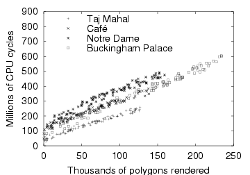
| The graph shows the CPU demand of rendering for four different scenes
at different resolutions (fidelities). For each scene, the camera
position was fixed arbitrarily. All experiments were run on the
hardware described in Section 4.1.
|
Figure 6: CPU demand of rendering (fixed camera, varying resolution)
Rendering is CPU-bound, and good interactive response depends on
accurate prediction and regulation of CPU demand. For our rendering
algorithm, resolution is the fidelity metric: thus we need to
know the mapping from resolution to CPU demand. CPU demand depends
both on the resolution r and the original polygon count p; from
examining the algorithm, we expected in fact that it would be a
function of pr, the rendered polygon count.
To map resolution to CPU demand, we started by logging the CPU demand
at different resolutions for four different scenes, and plotting CPU
demand against rendered polygon count
(Figure 6). We see that CPU demand is
linear in rendered polygon count:
for a fixed scene and camera position (note that different scenes have
different values of c0 and c1). However, the scene and the
camera position are parameters that can vary at runtime, and must be
tracked. In the following sections, we show how we track this
variation using data-specific prediction and online
learning.
3.4.2 Data-specific prediction
Sometimes resource demand depends on data-specific effects other than
the data size, which are not easily expressed as numeric
parameters. For example, the CPU demand of rendering depends on the
contents of the scene being rendered. In such cases, data-specific
prediction can be extremely useful: maintaining separate predictor
coefficients for each data objects. Sometimes, these can be computed
offline and stored with the data: for example, JPEG [36]
compression ratios depend on image content, and these
"compressibility coefficients" could be precomputed and stored at
the web server.
In other cases, the data-specific coefficients must be computed
online, after observing the resource demand of a few operations on a
new data object. This can still be useful if we perform many
operations on the same object: for example, with rendering, the user
will usually navigate a single scene for a while.
3.4.3 Online learning
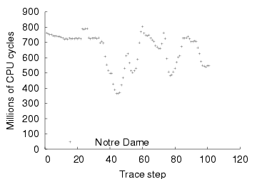
| The graph shows the CPU demand of rendering the Notre Dame scene over
time, at a resolution of 1. Each point corresponds to one camera
position in a motion trace of a user navigating the scene. All
experiments were run on the hardware described in
Section 4.1.
|
Figure 7: CPU demand of rendering (fixed resolution, moving camera)
Sometimes, we may have portions of application state which affect
resource demand but are not easily used as part of a predictive
model. For example, the CPU demand of rendering depends not only on
the resolution and the scene, but also on the camera
position. Figure 7 shows that the CPU demand of
rendering varies considerably with camera position as a user navigates
a scene, even when fidelity is fixed.
Thus, camera position and orientation are nontunable parameters
affecting CPU demand. Unfortunately, their effect on CPU demand is
very complex, depending on local properties of the scene: mapping them
directly to CPU demand requires large and expensive lookup tables.
Instead, we use a much simpler technique based on the observation that
- At each camera position, the linear relationship
Dcpu = c0 + c1pr holds, but c0 and c1 vary with camera
position.
- In typical use, camera position changes incrementally: the user
follows a continuous path through the scene.
- CPU demand has locality: a small change in camera position results
in a small change to c0 and c1.
We use an online-learning method that uses the linear mapping
Dcpu = c0 + c1pr, but continuously updates the values of c0
and c1 to reflect the behaviour corresponding to the current camera
position. We use recursive least-squares regression with exponential
decay [39], a modification of the well-known linear
regression method [18]. This gives greater weight to more
recent data by decaying the weight of data exponentially over
time. Our predictor uses a decay factor of 0.5, which makes it very
agile, effectively remembering only the last 4 data points. It is also
cheap: a 2-dimensional linear fit requires only tens of bytes of
state, and tens of floating point instructions per update.
The online-learning predictor is also data-specific. For each new
scene, it initializes a predictor with generic coefficients computed
from a variety of scenes and camera positions. Subsequent renders of
that scene result in updates of the scene-specific predictor,
specializing it both for the scene and the camera position within the
scene. In Section 4.3 we show that these two
simple techniques improve prediction accuracy significantly for
rendering; we believe that they have more general applicability as
well.
3.5 Utility functions
Utility functions represent a user's tradeoff policy between fidelity
and performance. Given some estimated fidelity and performance, the
utility function returns a number in [0,1] representing the
resulting user happiness; 0 represents the least possible user
satisfaction and 1 the most. By default, we use linear functions for
utility as a function of fidelity, and sigmoids for utility as a
function of latency. The product of these functions gives us a
multidimensional utility function whose range is still [0,1]. In
Odyssey, utility functions are computed by binary code modules; the
user can override the default utility function with an arbitrarily
general one by providing their own module.
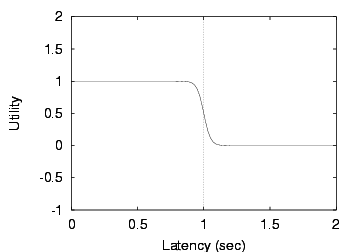 Figure 8: Sigmoid utility function
A sigmoid is a smoothed version of a step function. Instead of having
utility fall off a cliff when latency exceeds its target value, we can
now specify a tolerance zone where latency degrades linearly.
Figure 8 shows a sigmoid with a target of
1 s and a tolerance of 10%. There is little gain in utility
from decreasing latency below 0.9 s: this is the sweet
spot of the curve. Above 0.9 s, utility decreases steadily, and
latencies above 1.1 s are unacceptable to the user.
Figure 8: Sigmoid utility function
A sigmoid is a smoothed version of a step function. Instead of having
utility fall off a cliff when latency exceeds its target value, we can
now specify a tolerance zone where latency degrades linearly.
Figure 8 shows a sigmoid with a target of
1 s and a tolerance of 10%. There is little gain in utility
from decreasing latency below 0.9 s: this is the sweet
spot of the curve. Above 0.9 s, utility decreases steadily, and
latencies above 1.1 s are unacceptable to the user.
4 Evaluation
This section validates the predictive resource management approach by
answering three sets of questions:
- Is history-based demand prediction accurate? Are data-specific
prediction and online learning useful?
- How does predictive resource
management improve performance? Can multiple concurrent applications
adapt successfully without interfering with each other?
- What are the programming costs and runtime overhead of using the
system?
Before we describe the experiments that answer these questions, we
first describe our experimental setup
(Section 4.1) and evaluation metrics
(Section 4.2).
Sections 4.3-4.5 then
address each of the above sets of questions in turn.
4.1 Experimental platform and benchmarks
Our platform for all experiments reported in this paper is an IBM
ThinkPad 560 with a 233 MHz Mobile Pentium MMX processor,
96 MB of RAM, no 3-D graphics hardware, and running a standard
Linux 2.4.2 kernel. We used this rather than a wearable computer for
ease of development and testing; its processing power is comparable
with recent wearable and handheld platforms such as the IBM Linux
watch [29] and the Compaq iPAQ
3650.
Our motivating example - augmented reality - is not a mature
technology, and fully fledged AR applications are not freely
available. Instead, we use as benchmarks two applications -
GLVU and Radiator - which provide one component of AR:
3-D rendering. Together, these applications approximate the
augmented reality scenario of
Section 2.3: an architect using AR for
on-site design.
GLVU [35] is a "virtual walkthrough" program that
allows a user to explore a virtual 3-D scene: its function is to
render the scene from any viewpoint chosen by the user. In our
experiments, we simulate a moving user by replaying a trace of a user
navigating a 3-D scene using GLVU's graphical user
interface. We assume a continually moving user, and do not insert any
think times between render requests.
Radiator [38] computes lighting effects for 3-D rendering
using radiosity algorithms [8]. In an AR scenario, it would
be re-run whenever the user modified the scene lighting, for example
by adding a window to a building. We simulate this user behaviour by
running sporadic radiosity computations during the virtual
walkthrough, with random intervening think times.
Both GLVU and Radiator support multiresolution
scaling [17], which allows each render or radiosity
computation to be done at any resolution - any fraction of the
original polygon count. The overhead of changing the resolution is
negligible. Resolution is thus the single fidelity metric for both
computations.
In a real AR application, the user would be able to interactively edit
the scene, and the lighting effects computed by Radiator would be fed
back into GLVU for rendering. In our version, GLVU
and Radiator lack interactive editing facilities and do not
communicate with each other. However, the benchmarks are
representative of AR from a resource and performance point of view.
4.2 Evaluation metrics
Demand predictor accuracy is measured by running an application
benchmark on an unloaded system, and measuring the relative error for
each operation: the difference between the predicted and observed
resource demand, divided by the latter. We use relative rather than
absolute prediction error since it is applicable across a wide range
of values. Given the relative error for a number of operations, we
report the 90th percentile error E90. An E90 of 5%
means that 90% of the time, the predictor was within 5% of the
correct value.
Our metric of interactive application performance is operation
latency. Specifically, we measure Odyssey's ability to keep latency
within user-specified bounds, with low variability and without
unnecessarily sacrificing fidelity. In other words, we measure the
ability of the adaptive mechanism - Odyssey - to implement one
kind of policy: keeping latency steady. Our adaptive policies are
implemented by a sigmoidal utility function centred on the desired
latency bound (Section 3.5), with a tolerance of
10%. Utility also increases linearly with fidelity. The net effect is
that utility is maximized at 90% of the latency bound: this is the
target latency.
We conduct 5 trials of each experimental run. For each such set of 5
trials, we report the mean operation latency, and also the coefficient
of variation: the standard deviation of latency divided by the mean.
In some cases, we also show a timeline of one of the trials, to
illustrate the performance and fidelity over time.
Ideally, we want mean latency to be on target. Higher latencies
indicate bad interactive response, while lower latencies indicate an
unnecessary sacrifice of fidelity. We also want the coefficient of
variation to be small: variability in performance leads to a bad user
experience [24]. High variation also indicates that the
system is often off-target: in other words, not implementing the
adaptive policy well.
4.3 Demand predictor accuracy
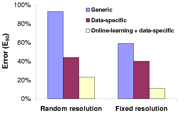
| We show 90th percentile error (in %) of three different schemes for
predicting the CPU demand of rendering. The CPU demand itself varies
between 0.1 s and 5 s (23-1018 million cycles).
|
Figure 9: CPU demand prediction error for rendering
In this section, we show that history-based demand predictors provide
accurate predictions across a range of applications and resources.
For brevity, we describe in detail only the CPU demand predictor for
GLVU, and summarize results for other predictors.
For GLVU, we measured the accuracy of the data-specific,
online-learning predictor, and also the contribution of
data-specificity and online learning to this accuracy. We compared
- a generic predictor, which fits a single pair of
coefficients c0, c1 to all 4 scenes,
- a data-specific predictor, which specializes c0 and c1
to each scene,
- the online-learning predictor, which maintains
scene-specific coefficients, and also updates them after each
operation to track runtime variation in CPU demand.
The accuracy of CPU demand prediction depends not only on the
variation in camera position, but also on the variation in fidelity
from one rendering operation to the next. In an adaptive system,
variation in fidelity is driven by variation in resource supply at
runtime. To estimate demand prediction accuracy independent of
runtime conditions, we evaluated both the worst case of randomly
varying fidelity and the best case of fixed fidelity.
Figure 9 shows the prediction error of these three
predictors for both random and fixed resolution (1.0), measured on
user traces on four different scenes. Each trace has 100 camera
positions, yielding 400 data points in all. We see that both
data-specificity and online learning decrease prediction error. The
best predictor, online-learning, has a worst-case error of 24%, which
is small compared to the order-of-magnitude variation in CPU demand.
Better learning techniques could improve its accuracy further.
| Application | Tunable | Resource | Observed range | Data | Online | E90 |
| parameters | | of resource demand | specific? | learning? | |
| GLVU | Resolution | CPU | 23-1018 | Mcycles | Yes | Yes | 24% |
| Radiator | Resolution, | Memory | 14-60 | MB | No | No | 3% |
| algorithm | CPU | 220-46219 | Mcycles | Yes | No | 11% |
| Web browser | JPEG level | Energy | 1.5-25 | Joules | Yes | No | 9% |
| Speech | Client-server | Network | 4-219 | KB | No | No | 0.3% |
| recognizer | split, vocab. | client CPU | 0-2774 | Mcycles | No | No | 10% |
| size | server CPU | 0-2128 | Mcycles | No | No | 16% |
| The table shows the 90th percentile error E90 (right-most column)
of history-based demand predictors for different applications and
resources. In each case, we also show the observed min-max range of
resource demand, measured in millions of cycles of CPU, megabytes of
memory, Joules of energy, or kilobytes of network
transmission/reception.
|
Figure 10: Demand predictor accuracy for various applications and resources
We also measured demand predictor accuracy for other applications -
Radiator, speech recognition, and web browsing - and other resources
- memory, network, and battery energy
(Figure 10). In each case, we are able to predict to
within a small fraction a quantity with a large dynamic range, showing
that multi-fidelity computation can make a big difference to resource
demand, and that we can predict resource demand to within a small
error. Note that all the other predictors have better accuracy than
the CPU predictor for GLVU: our chosen example case study
represents our worst observed case.
4.4 Performance benefits
4.4.1 Single application with background load
 Fully adaptive
 Demand-only
 Static
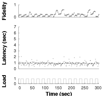
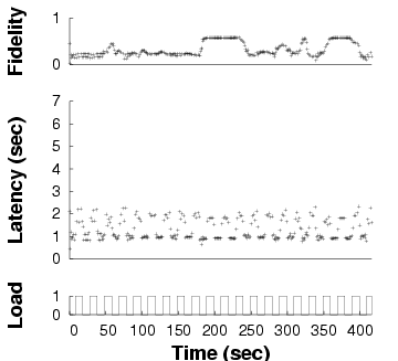
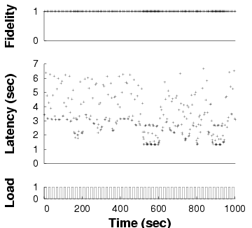
| Fidelity and latency of GLVU over time when subjected to a
time-varying background load, in three different adaptation
configurations. Note the different time scales on the x axes: the same
benchmark takes different amounts of time in different configurations.
|
Figure 11: Adaptation in GLVU
Given that demand prediction is accurate, what is the impact on
performance of predictive resource management? To answer this
question, we measured the performance of GLVU adapting
dynamically to changes in resource supply. GLVU plays a
trace of a user navigating the "Notre Dame" scene, while Odyssey
attempts to bound operation latency to 1 s. Simultaneously, a
competing process alternates between spinning and sleeping every
10 s. We chose this square waveform over more realistic load
patterns to explore the effect of load frequency and amplitude.
We ran this experiment in three configurations:
- Fully adaptive: both supply and demand
prediction are enabled, so GLVU adapts to changes both in
application demand and in background load.
- Demand-only: we enable CPU demand prediction,
which allows GLVU to regulate its CPU demand to the target
value. However, supply prediction is disabled: the background load is
assumed to be 0.
- Static: GLVU's fidelity is fixed at 1: there
is no adaptation at all.
Figure 11 shows one run for each configuration,
in our baseline case: a trace of "Notre Dame" with a 1 s
latency bound, a 0.1 Hz background load frequency, and a peak
load of 1. We see that the "fully adaptive" configuration keeps
latency on target. "Demand-only" is on target only when unloaded,
and "static" almost never. Note that the different experiments have
different run times, the effect of reducing mean latency on a
fixed-work benchmark.
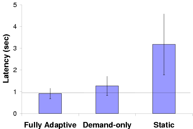 Mean latency
 Variability in latency
| Error bars show standard deviations; the horizontal line marks the
target latency.
|
Figure 12: Adaptive performance in GLVU
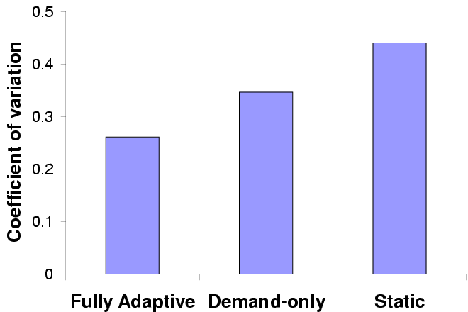
Figure 12 shows mean latency and variation over
5 trials for each configuration. We see that demand prediction alone
substantially improves interactive performance by bringing mean
latency close to the target value and reducing variability; supply
prediction improves performance further.
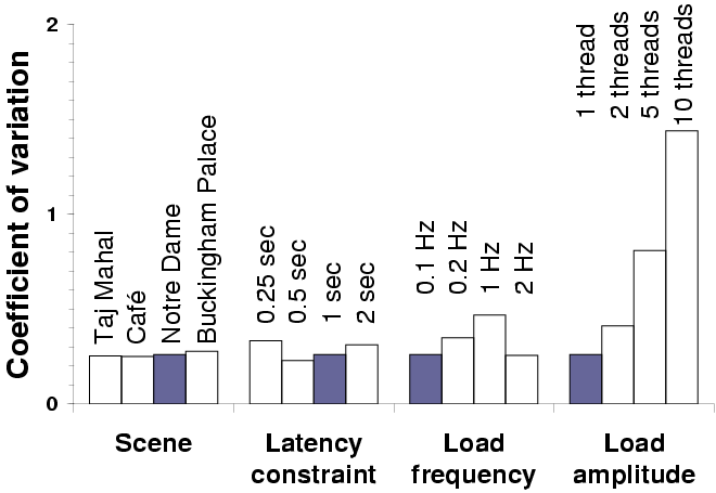
| The graph shows the coefficient of variation for latency under various
experimental conditions. Each set of bars varies one parameter: the
shaded bars represent the baseline case.
|
Figure 13: GLVU adaptation: sensitivity analysis
To validate our results across a range of experimental parameters, we
tested the "fully adaptive" configuration with different 3-D
scenes, latency bounds, and load patterns. In each case, we varied
one parameter, keeping the others fixed, and compared the performance
against the baseline case: Figure 13 shows
the results of these experiments.
Mean latency was insensitive to experimental parameters, except when
we reduced the latency bound to 0.25 s: in this case mean
latency exceeds target by 20%. Here we hit the limit of fidelity
degradation: on our test platform, rendering can take up to
0.46 s of CPU time even at the lowest fidelity.
Variability in latency was the same for all scenes, but varied with
other parameters. Variability was lowest for a 0.5 s latency
bound. At lower latencies, Linux's 200 ms scheduler quantum
causes variability. At higher latencies, load transitions are more
frequent with respect to operation rate, causing more operations to
deviate from target.
Variability was highest when load frequency matched operation rate
(1 Hz). At lower frequencies, fewer operations are hit by load
transitions. At higher frequencies, load variation gets smoothed out
over the course of an operation. Variability also increases sharply
with increasing load amplitude (peak-to-trough difference): operations
hit by load transitions are more affected by larger transitions.
We observe that it is most important to predict resource supply
at the time scale of adaptation: higher and lower frequencies impact
latency less. If this time scale is comparable to the scheduler
granularity, then prediction accuracy will be low and performance
variability will be high.
4.4.2 Concurrent applications
When we run two adaptive applications concurrently, are they both able
to adapt effectively, or do they interfere with each other's
performance? To answer this question, we mimicked an AR scenario by
running GLVU and Radiator concurrently as Linux processes at
default priority.
GLVU replays a trace of a user navigating the virtual "Notre Dame"
scene. Meanwhile, Radiator runs sporadic radiosity computations on a
copy of the same scene in the background, to simulate occasional
re-computation of lighting effects by the user. Between operations,
Radiator sleeps for a random "think time" from 0-10 s. The
system's goal is to maintain the latency bounds of both applications
despite resource variation. We use a 1 s latency bound for
GLVU, as before. Radiator is much more resource-intensive,
and runs in the background: for it, we use a 10 s bound. For
both applications, we use a sigmoid utility function with a 10%
tolerance (Section 3.5): thus, the sweet spot or
target latency is 0.9 s for GLVU and 9 s for
Radiator.
We ran this experiment in 5 configurations:
- Adaptive-both: both applications adapt fidelity to achieve the
target latency.
- Static-optimal: fidelity is static, but tuned for this
benchmark. We set it to the mean fidelity achieved in the adaptive
case (0.17 for GLVU, 0.019 for Radiator).
- Static-user: fidelity is static, at 0.5 for GLVU
and 0.05 for Radiator: reasonable values that a user might select
without workload-specific tuning.
- Adaptive- GLVU: GLVU adapts, Radiator
uses the "static-user" fidelity.
- Adaptive-Radiator: Radiator adapts, GLVU
uses the "static-user" fidelity.
The last two configurations represent real-world cases where one
application is modified with multi-fidelity support, but the other is
unmodified and must rely on the user to set the fidelity.
 Adaptive-both
 Static-optimal
 Static-user
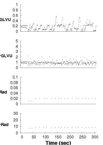
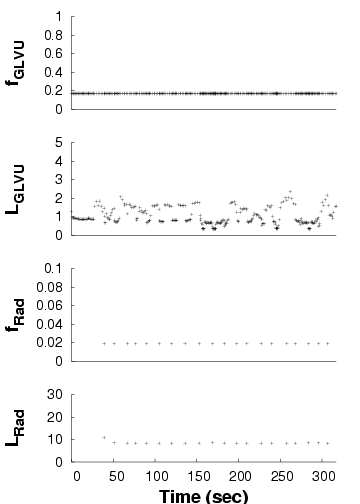
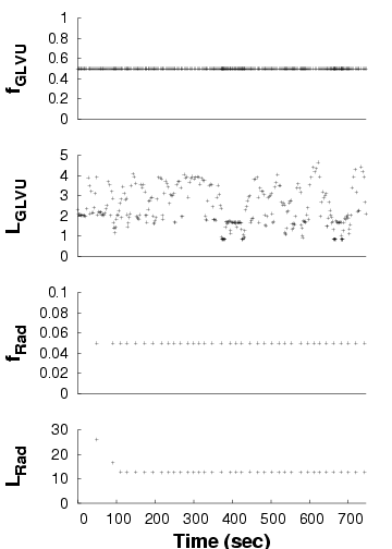
| We show the performance of concurrent applications ( GLVU and
Radiator) over time, in three configurations. Each graph shows a time
line of GLVU's fidelity (fGLVU), GLVU's latency
in seconds (LGLVU), Radiator's fidelity (fRad), and
Radiator's latency in seconds (LRad). Note the different time
scale for the "static-user" graph. For lack of space, we omit the
timelines for the "adaptive- GLVU" and "adaptive-Radiator"
timelines: the adaptive and non-adaptive performance in these cases is
very similar to that shown for the "adaptive-both" and
"static-user" cases.
|
Figure 14: Adaptation in concurrent applications
Figure 14 shows one trial each for the
first three configurations. In the "adaptive-both" case,
GLVU maintains its target latency despite supply and
demand variation. With "static-optimal", mean latency is on target
but variability is high; with "static-user", mean latency is off
target and variability is even higher.
For Radiator, "adaptive-both" and "static-optimal" get latency on
target, while "static-user" is off target. Variability is low in all
cases: Radiator's CPU demand is invariant with time and camera
position. CPU supply does not vary either: at 10 s time scales,
the competing load imposed by
GLVU is constant. "Static-optimal" has slightly lower
variability than "adaptive", which executes a few operations at the
wrong fidelity before converging on the correct value.
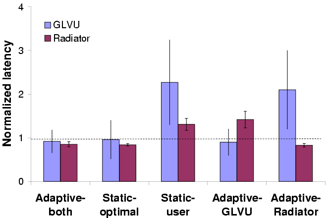 Mean normalized latency
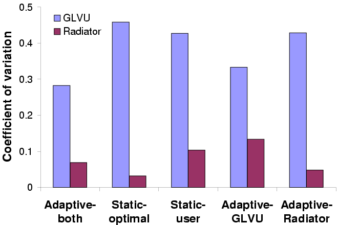 Variability in latency
| Error bars show standard deviations; the horizontal line marks the
target latency.
|
Figure 15: Adaptive performance for concurrent applications
Figure 15 shows the mean normalized latency
(latency divided by the latency bound) and coefficient of variation
over 5 trials of all 5 configurations. We see that adaptation keeps
latency on target without any workload-specific tuning, and reduces
variation. Workload-specific tuning ("static-optimal") can get mean
latency on target, but cannot prevent dynamic variation due to changes
in resource supply or demand. Adaptation also insulates each
application's performance from the other's: the
"Adaptive- GLVU" and "Adaptive-Radiator" graphs show that
the benefit gained from adaptation is independent of the other
application's behavior. In other words, our approach can be useful
even without a coordinated effort to modify all running
applications. This is a valuable property for real-world deployment.
4.5 Costs and overheads
4.5.1 Porting costs
The cost of porting legacy applications to a new API is an important
measure of system deployability. Figure 16 shows
the amount of source code modification required for four applications
to use the multi-fidelity API. Three of these already had the
potential for fidelity adaptation: for example, Radiator comes with
support for multiresolution models. GLVU had to be augmented
with multiresolution support, and we include the cost of this step.
Multi-fidelity support requires 500-1000 new or modified lines of
code, including the ACF and hint module: a modest investment of
programmer effort. Many of these lines are in glue code between
application constructs and the generic multi-fidelity API. We are
investigating the use of stub generators to automatically generate
this glue code.
4.5.2 Runtime overheads
| Application | Original size | Modifications |
| KLOCf | Files | KLOCf | Files |
| GLVU | 27.0 | 144 | 0.9f | 7f |
| Radiator | 51.1 | 222 | 0.6 | 5 |
| Web proxy | 3.9 | 9 | 0.9 | 6 |
| Speech recognizer | 126.4 | 209 | 1.1 | 10 |
f 1 KLOC = 1000 lines of code
f Includes multiresolution support (0.4 KLOC, 2 files)
|
Figure 16: Cost of porting legacy code
| Component | Overhead |
| App-Odyssey communication | 0.36 ms |
| Logger (buffered at user level) | 0.15 ms |
| Logger (unbuffered) | 0.20 ms |
| CPU supply/demand monitor | 1.38 ms |
| Memory supply/demand monitor | 6.72 ms |
| Solver | 10.56 ms |
| Total | 19.37 ms |
Figure 17: Per-operation runtime overhead
Figure 17 shows the overhead of each runtime
component in additional latency per operation for a synthetic
benchmark. The total overhead is around 20 ms: only 2% for a
1 s operation, but an unacceptable 20% for a 100 ms
latency bound. We are looking at reducing the overheads by using a
more efficient and scalable solver; with better interfaces for load and
resource statistics (/proc contributes most of the latency to
our resource predictors); and by replacing the middleware server with
a library implementation.
5 Related work
This work is most closely related to previous work on fidelity
adaptation [7,9,16,15,30]. We
have generalized these previous notions of fidelity, which only
measured data degradation, to include arbitrary runtime parameters of
an application. Our system and API also move the burden of adaptation
out of the application: where other systems expect applications to
specify their resource requirements, we predict resource supply,
demand, and performance based on observations of history. Although
resource demand prediction is still application-specific, it has been
cleanly separated from the rest of the system, and our history-based
methodology and measurement/logging infrastructure make it an easier
task than before.
We also diverge from traditional models of adaptation by using a
predictive rather than a feedback-driven approach. Rather than
adjusting fidelity in small steps in response to a change in
performance, Odyssey can make large yet accurate adaptations in a
single step. This is made possible by Odyssey's ability to predict
supply, demand and performance across the entire range of fidelities.
Related, but complementary to application adaptation is work on
QoS-based reservations [26,22] and remote
execution [13,4]: Section 2.1
discussed these in more detail.
Also related is previous work on resource prediction. Supply
prediction - predicting load from past measurements - is present
in many systems. Usually it is present implicitly in a feedback loop:
measurements of load or performance are used as control signals to
adjust system parameters [34]. A few systems use explicit
prediction of load: for example, Dinda's Running Time
Advisor [10]. Explicit prediction of resource demand,
however, is comparatively rare. Most systems assume that resource
demand is constant, specified by the application, derived from a
static probability distribution [23,19], or
obtained from compile-time analysis [33].
We know of two systems that explicitly predict resource demand as a
function of runtime parameters: however, neither uses the predictions
for application adaptation. Automated profiling for
QoS [1] estimates the CPU utilization of a multimedia
stream as a linear function of task rate and task size, for admission
control purposes. PUNCH [21] uses machine learning to
predict CPU demand as a function of application-specific runtime
parameters, for load-balancing in a grid framework. To the best of our
knowledge, Odyssey is the first system to use history-based prediction
to model resource demand as a function of fidelity in adaptive
applications.
6 Conclusion
We have shown in this paper that multi-fidelity computation supported
by predictive resource management can improve performance in mobile
interactive applications. Our performance evaluation shows that
- We reduce mean latency by 60% and variability by 30%
for GLVU subjected to a time-varying load.
- History-based demand prediction is accurate and effective,
with prediction errors as low as 0.3% for some resources and never
higher than 24% in our case studies.
- The cost of using Odyssey is modest, involving 500-1000 additional
lines of code per application and 20 ms of runtime overhead per
interactive operation.
Throughout the paper, we have indicated areas for incremental
improvement; here we mention a few medium to long-term goals for
future research. We would like to test Odyssey with a full-fledged AR
application on wearable hardware, including location tracking and
machine vision as well as rendering, and 100 ms latency bounds
rather than 1 s. We would like to further automate the
construction of demand predictors: for example, by building
platform-independent CPU predictors that can be used across processor
architectures. We would like to combine demand prediction with
QoS-based allocation such that the system can simultaneously optimize
allocation across, and adaptation within,
applications [31]. Finally, we would like to explore
mixed-initiative [20] approaches that combine direct user
modification of utility functions with automated inference by the
system about user preferences.
References
- [1]
-
T. F. Abdelzaher.
An Automated Profiling Subsystem for QoS-Aware Services.
In Proc. 6th IEEE Real-Time Technology and Applications
Symposium (RTAS '00), pages 208-217, Washington, DC, June 2000.
- [2]
-
A. Arpaci-Dusseau and R. Arpaci-Dusseau.
Information and Control in Gray-Box Systems.
In Proc. 18th ACM Symposium on Operating Systems Principles
(SOSP 2001), pages 43-56, Chateau Lake Louise, Banff, Canada, Oct. 2001.
- [3]
-
R. Azuma, Y. Baillot, R. Behringer, S. Feiner, S. Julier, and B. MacIntyre.
Recent Advances in Augmented Reality.
IEEE Computer Graphics and Applications, 21(6):34-47,
Nov. Dec. 2001.
- [4]
-
R. K. Balan, M. Satyanarayanan, S. Park, and T. Okoshi.
Tactics-Based Remote Execution for Mobile Computing.
In Proc. 1st International Conference on Mobile Systems,
Applications, and Services (MobiSys '03), San Francisco, CA, May 2003.
- [5]
-
M. Billinghurst, S. Weghorst, and T. A. Furness.
Wearable Computers for Three Dimensional CSCW.
In Proc. International Symposium on Wearable Computers, pages
39-46, Cambridge, MA, Oct. 1997.
- [6]
-
S. Chandra and C. Ellis.
JPEG Compression Metric as a Quality Aware Image Transcoding.
In Proc. 2nd USENIX Symposium on Internet Technologies and
Systems (USITS '99), pages 81-92, Boulder, CO, Oct. 1999.
- [7]
-
S. Chandra, C. Ellis, and A. Vahdat.
Differentiated Multimedia Web Services Using Quality Aware
Transcoding.
In Proc. 19th Annual Joint Conference of the IEEE Computer and
Communications Societies. Proceedings (INFOCOM '00), pages 961-969, Tel
Aviv, Israel, Mar. 2000.
- [8]
-
M. F. Cohen and J. R. Wallace.
Radiosity and Realistic Image Synthesis.
Academic Press Professional, Boston, MA, 1993.
- [9]
-
E. de Lara, D. S. Wallach, and W. Zwaenepoel.
Puppeteer: Component-based Adaptation for Mobile Computing.
In Proc. 3rd USENIX Symposium on Internet Technologies and
Systems (USITS-01), pages 159-170, Berkeley, CA, Mar. 2001.
- [10]
-
P. A. Dinda.
Online Prediction of the Running Time of Tasks.
In Proc. 10th IEEE International Symposium on High Performance
Distributed Computing (HPDC '01), pages 383-394, San Francisco, CA, Aug.
2001.
- [11]
-
A. H. Dutoit, O. Creighton, G. Klinker, R. Kobylinski, C. Vilsmeier, and
B. Bruegge.
Architectural Issues in Mobile Augmented Reality Systems: a
prototyping case study.
In Proc. Eighth Asian Pacific Conference on Software Engineering
(APSEC'2001), pages 341-344, Macau, China, Dec. 2001.
- [12]
-
S. Feiner, B. MacIntyre, T. Höllerer, and A. Webster.
A Touring Machine: Prototyping 3D Mobile Augmented Reality
Systems for Exploring the Urban Environment.
In Proc. International Symposium on Wearable Computers, pages
74-81, Cambridge, MA, Oct. 1997.
- [13]
-
J. Flinn, D. Narayanan, and M. Satyanarayanan.
Self-Tuned Remote Execution for Pervasive Computing.
In Proc. 8th Workshop on Hot Topics in Operating Systems
(HotOS-VIII), pages 61-66, Schloss Elmau, Germany, May 2001.
- [14]
-
J. Flinn, S. Park, and M. Satyanarayanan.
Balancing Performance, Energy, and Quality in Pervasive Computing.
In Proc. 22nd International Conference on Distributed Computing
Systems (ICDCS '02), pages 217-226, Vienna, Austria, July 2002.
- [15]
-
J. Flinn and M. Satyanarayanan.
Energy-Aware Adaptation for Mobile Applications.
In Proc. 17th ACM Symposium on Operating Systems Principles
(SOSP '99), pages 48-63, Kiawah Island, SC, Dec. 1999.
- [16]
-
A. Fox, S. D. Gribble, E. A. Brewer, and E. Amir.
Adapting to Network and Client Variability via On-Demand Dynamic
Distillation.
In Proc. 7th International Conference on Architectural Support
for Programming Languages and Operating Systems (ASPLOS '96), pages
160-170, Cambridge, MA, Oct. 1996.
- [17]
-
M. Garland and P. S. Heckbert.
Surface Simplification Using Quadric Error Metrics.
In Proc. SIGGRAPH '97, pages 209-216, Los Angeles, CA, Aug.
1997.
- [18]
-
C. F. Gauss.
Theoria Combinationis Observationum Erroribus Minimum
Obnoxiae.
Royal Society of Göttingen, 1821.
- [19]
-
M. Harchol-Balter and A. B. Downey.
Exploiting Process Lifetime Distributions for Dynamic Load
Balancing.
In Proc. Joint International Conference on Measurement and
Modeling of Computer Systems (ACM SIGMETRICS '94), pages 13-24, Nashville,
TN, May 1994.
- [20]
-
E. Horvitz.
Principles of Mixed-Initiative User Interfaces.
In Proc. ACM SIGCHI Conference on Human Factors in Computing
Systems (CHI '99), pages 159-166, Pittsburgh, PA, May 1999.
- [21]
-
N. H. Kapadia, J. A. B. Fortes, and C. E. Brodley.
Predictive Application-Performance Modeling in a Computational Grid
Environment.
In Proc. 8th IEEE International Symposium on High Performance
Distributed Computing (HPDC '99), pages 47-54, Los Angeles, CA, Aug. 1999.
- [22]
-
C. Lee, J. Lehoczky, D. Siewiorek, R. Rajkumar, and J. Hansen.
A Scalable Solution to the Multi-Resource QoS Problem.
In Proc. 20th IEEE Real-Time Systems Symposium (RTSS '99),
pages 315-326, Phoenix, AZ, Dec. 1999.
- [23]
-
W. E. Leland and T. J. Ott.
Load-balancing Heuristics and Process Behavior.
In Proc. Joint International Conference on Measurement and
Modeling of Computer Systems (ACM SIGMETRICS '86), pages 54-69, Raleigh,
NC, May 1986.
- [24]
-
R. B. Miller.
Response Time in Man-Computer Conversational Transactions.
AFIPS Fall Joint Computer Conference Proceedings, 33:267-277,
Dec. 1968.
- [25]
-
D. J. Musliner, E. H. Durfee, and K. G. Shin.
Any-Dimension Algorithms.
In Proc. 9th IEEE Workshop on Real-Time Operating Systems and
Software (RTOSS '92), pages 78-81, May 1992.
- [26]
-
K. Nahrstedt, D. Xu, D. Wichadukul, and B. Li.
QoS-Aware Middleware for Ubiquitous and Heterogeneous
Environments.
IEEE Communications, 39(11):140-148, Nov. 2001.
- [27]
-
D. Narayanan.
Operating System Support for Mobile Interactive Applications.
PhD thesis, Carnegie Mellon University, Aug. 2002.
- [28]
-
D. Narayanan, J. Flinn, and M. Satyanarayanan.
Using History to Improve Mobile Application Adaptation.
In Proc. 3rd IEEE Workshop on Mobile Computing Systems and
Applicatons, pages 31-40, Monterey, CA, Dec. 2000.
- [29]
-
C. Narayanaswami, N. Kamijoh, M. Raghunath, T. Inoue, T. Cipolla, J. Sanford,
E. Schlig, S. Venkiteswaran, D. Guniguntala, V. Kulkarni, and K. Yamazaki.
IBM's Linux watch, the challenge of miniaturization.
IEEE Computer, 35(1):33-41, Jan. 2002.
- [30]
-
B. D. Noble, M. Satyanarayanan, D. Narayanan, J. E. Tilton, J. Flinn, and K. R.
Walker.
Agile Application-Aware Adaptation for Mobility.
In Proc. 16th ACM Symposium on Operating Systems Principles
(SOSP '97), pages 276-287, Saint Malo, France, Oct. 1997.
- [31]
-
D. Petrou and D. Narayanan.
Position Summary: Hinting for Goodness' Sake.
In Proc. 8th Workshop on Hot Topics in Operating Systems
(HotOS-VIII), page 177, Schloss Elmau, Germany, May 2001.
- [32]
-
M. Satyanarayanan and D. Narayanan.
Multi-Fidelity Algorithms for Interactive Mobile Applications.
Wireless Networks, 7:601-607, 2001.
- [33]
-
B. S. Siegell and P. Steenkiste.
Automatic Generation of Parallel Programs with Dynamic Load
Balancing.
In Proc. 3rd IEEE International Symposium on High Performance
Distributed Computing (HPDC '94), pages 166-175, San Francisco, CA, Aug.
1994.
- [34]
-
D. C. Steere, A. Goel, J. Gruenberg, D. McNamee, C. Pu, and J. Walpole.
A Feedback-Driven Proportion Allocator for Real-Rate Scheduling.
In Proc. 3rd Symposium on Operating Systems Design and
Implementation (OSDI '99), pages 145-158, New Orleans, LA, Feb. 1999.
- [35]
-
The Walkthru Project.
GLVU source code and online documentation.
https://www.cs.unc.edu/~walk/software/glvu/, Feb. 2002.
- [36]
-
G. K. Wallace.
The JPEG still picture compression standard.
Communications of the ACM, 34(4):30-44, Apr. 1991.
- [37]
-
A. Webster, S. Feiner, B. MacIntyre, W. Massie, and T. Krueger.
Augmented Reality in Architectural Construction, Inspection and
Renovation.
In Proc. ASCE Third Congress on Computing in Civil Engineering,
pages 913-919, Anaheim, CA, June 1996.
- [38]
-
A. J. Willmott.
Radiator source code and online documentation.
https://www.cs.cmu.edu/~ajw/software/, Oct. 1999.
- [39]
-
P. Young.
Recursive Estimation and Time-Series Analysis.
Springer, 1984.
File translated from
TEX
by
TTH,
version 3.32.
On 5 Mar 2003, 10:28.
|
