Guanhua Yan![[*]](footnote.png)
Information Sciences (CCS-3)
Los Alamos National Laboratory
Los Alamos, NM 87545, USA
ghyan@lanl.gov
Zhen Xiao
School of Electronics Engineering and Computer Science
Peking University
Beijing, P. R. China
xiaozhen@net.pku.edu.cn
Stephan Eidenbenz
Information Sciences (CCS-3)
Los Alamos National Laboratory
Los Alamos, NM 87545, USA
eidenben@lanl.gov
Instant messaging (IM) systems have grown tremendously in the past few years. It is estimated that the total number of active IM accounts will increase from 867 million by the end of 2005 to 1.2 billion by 2009 [5] and the number of enterprise IM users will increase from 67 million in 2007 to 127 million in 2011 [6]. Accompanied with such increasing popularity of IM systems is the growing security threat that IM malware poses to both residential and enterprise IM users. For instance, from January 1, 2005 through September 2005, more than 360 new IM worms have surfaced [8]. According to a report from Akonix Systems Inc., there have been 346 IM attacks in 2007 [4]. In 2005, Reuters was even forced to shut down its instant messaging service temporarily due to the Kelvir IM worm [16].
IM worms have posed significant challenges to security protection for enterprise-like networks. IM worms can be leveraged to implant rootkits or bots onto victim machines inside an enterprise network after traditional perimeter protections such as firewalls have been bypassed. The two major propagation vectors of IM worms are file transfers and URL-embedded chat messages. An IM worm using the first approach (e.g., Sumom.a [19]) requests transferring a file, which contains the worm code, to an online buddy; in the second approach, an IM worm (e.g., Kelvir.k [7]) sends a hyperlink, which is embedded in a text chat message, to an online buddy. If the receiver accepts the file transfer request or clicks the embedded URL, a malicious file will be downloaded onto her machine and its execution creates a new infection.
Outbreaks of traditional Internet worms such as Code Red tell us that any effective defense scheme against an epidemic spreading requires a fast and responsive alert system [18]. Motivated by this, we propose to apply change-point detection techniques to detect two families of IM worms quickly. The first family of IM worms aim to infect all vulnerable machines as quickly as possible by aggressively hunting for new victims. We detect this type of IM worms by monitoring abrupt increase of file transfer requests or URL-embedded chat messages in the IM system. The second family of IM worms allow only a limited number of infection attempts within a certain period of time. Although spreading more slowly, this type of IM worms do not trigger a large number of file transfer requests or URL-embedded chat messages. Our detection scheme relies on the observation that different degrees of social online intimacy among IM buddies lead to uneven communication messages exchanged among them. An IM worm that randomly chooses online buddies as infection victims can, very likely, generate file transfer requests or URL-embedded chat messages between IM buddies that barely chat in the past. To detect this type of IM worms, we measure the average log-likelihood of file transfer requests or URL-embedded chat messages in the IM system; its abrupt decrease is a good indication of stealthy IM worm propagation. We evaluate our detection schemes with an IM dataset collected from a large enterprise network and experimental results show that they are very effective in detecting both families of IM worms.
The remainder of this paper is organized as follows. Section II presents some background knowledge about IM architecture and IM worms. Section III discusses IM worms that aggressively scan for new victims and their detection. Section IV discusses how an intelligent IM worm evades the detection scheme described in Section III. In this section, we also provide an algorithm that detects this type of IM worms. In Section V, we evaluate the effectiveness of the proposed solutions with an IM dataset collected from a large corporate network. We present some related work in Section VI and conclude this paper in Section VII.
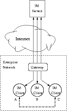
IM architectures. Popular IM systems include MSN messenger, AIM, Yahoo Messenger, IRC, ICQ, and Google Talk. Although these systems are built on different protocols, they bear little difference in their basic client-server structures. The general framework of an IM system in an enterprise-like network is depicted in Fig. 1. IM servers form the backbone of an IM system and their typical functionalities include account management, user authentication, presence notification, text-based chat message relaying, file transfer establishment, and group chatting. Albeit major IM systems provide similar functionalities, their server architectures may differ from each other. For instance, a text-based chat message in the AIM system has to go through two BOS (Basic Oscar Services) servers before it is delivered to the receiver, but a similar message in the MSN system traverses only one SB (switchboard) server [23].
In our work, we focus on schemes that detect IM worm propagation in a centralized fashion. More specifically, we consider approaches that can be directly deployed at the IM servers, or at the enterprise gateway if the goal is to protect an enterprise network. The feasibility of such a solution requires further explanation. Encryption is rarely used in existing major IM systems, suggesting IM servers or enterprise gateways can see most text-based chat messages delivered through them. Hence, if an IM worm uses the URL-embedded chat messages to spread itself, the IM servers or the enterprise gateway can parse unencrypted chat messages and derive the URL information. However, the IM servers or the enterprise gateway can not capture the file being transferred between two IM clients, unless the sender and receiver are both protected by a firewall or NAT router [23]. Hence, if an IM worm propagates through file transfers, we may not be able to detect IM worm propagation through binary malware code analysis at the enterprise gateway or the IM servers. Nevertheless, any file transfer between two IM clients must involve some IM servers to set up their initial connection, so we can still infer that a file transfer is going to take place between two IM clients by analyzing IM command traffic at the enterprise gateway or the IM servers.
IM worms. An infection attempt through an IM network consists of
two processes: handshaking and downloading. In the
handshaking step, an infected machine with IM account ![]() requests a
file transfer or sends a URL-embedded chat message to
requests a
file transfer or sends a URL-embedded chat message to ![]() 's online
buddy
's online
buddy ![]() . When IM user
. When IM user ![]() receives the file transfer request or the
URL-embedded chat message, she decides whether to accept the request
or click on the URL. Only if she does so will the next step take
place: the recipient machine downloads the worm code body from the
machine that
receives the file transfer request or the
URL-embedded chat message, she decides whether to accept the request
or click on the URL. Only if she does so will the next step take
place: the recipient machine downloads the worm code body from the
machine that ![]() is using if the file transfer scheme is used, or from
the host specified by the URL if the worm spreads by URL-embedded chat
messages. Once the second step finishes, the recipient machine gets
infected if it is vulnerable to the worm infection; otherwise, the
infection attempt fails.
is using if the file transfer scheme is used, or from
the host specified by the URL if the worm spreads by URL-embedded chat
messages. Once the second step finishes, the recipient machine gets
infected if it is vulnerable to the worm infection; otherwise, the
infection attempt fails.
We use ![]() and
and ![]() to denote the durations of the handshaking
step and the downloading step, respectively. We also use
to denote the durations of the handshaking
step and the downloading step, respectively. We also use ![]() to
denote the time needed to execute the worm code on a victim machine,
e.g., modifying the registry on a Windows machine. Let
to
denote the time needed to execute the worm code on a victim machine,
e.g., modifying the registry on a Windows machine. Let ![]() be the
probability that a node accepts a file transfer request or clicks on
the embedded URL.
be the
probability that a node accepts a file transfer request or clicks on
the embedded URL. ![]() essentially reflects the probability that the
worm spreading attempt succeeds in each hop. We also use
essentially reflects the probability that the
worm spreading attempt succeeds in each hop. We also use ![]() to
denote the probability that a node is vulnerable to the worm infection
after the worm code body is downloaded.
to
denote the probability that a node is vulnerable to the worm infection
after the worm code body is downloaded.
Many existing IM worms adopt the fast scanning strategy, that is, they, after infecting a new host, immediately iterate the online buddy list and attempt to infect each contact on it either by requesting a file transfer or sending out a URL-embedded chat message. Such IM worms include Bropia and Kelvir that have been observed spreading on the MSN IM network. The common objective of fast scanning IM worms is to infect all vulnerable machines as quickly as possible. Experiences with traditional Internet worms such as Code Red and Slammer suggest that an effective defense scheme against a fast scanning worm must detect it at its early propagation stage [18].
Algorithm description. The aggressive spreading strategy used
by fast scanning IM worms, although accelerating their propagation,
inevitably increases the number of file transfer requests or
URL-embedded chat messages in the IM systems, depending on their
infection vectors. Moreover, these file transfer requests or
URL-embedded text messages introduced by fast scanning IM worms bear
different source-destination pairs. Such a distinguishing feature of
fast scanning IM worms motivates us to apply sequential change
detection theory for their detection. The key idea of sequential
change detection theory is to locate the point of change, if it
occurs, within an observed time series by checking whether it is
statistically homogeneous in an online fashion. Further explanation
requires more notations. We discretize time into measurement windows
of equal length ![]() , denoted by
, denoted by
![]() . We use random sequence
. We use random sequence
![]() and
and
![]() to
denote the total number of file transfer requests and URL-embedded
chat messages with different source-destination pairs that have been
observed within the
to
denote the total number of file transfer requests and URL-embedded
chat messages with different source-destination pairs that have been
observed within the ![]() -th measurement window, respectively.
-th measurement window, respectively.
To detect fast scanning IM worms, we use the CUSUM algorithm
[14], which is a standard tool in statistical process
control. Particularly, we apply its non-parametric version
[1] as it does not demand any a
priori information on distributions of the random sequence before
and/or after the change point. Let
![]() be a random sequence with mean
be a random sequence with mean ![]() under normal operation. Our
goal is to detect whether there is an abrupt change of mean in
under normal operation. Our
goal is to detect whether there is an abrupt change of mean in ![]() . As the non-parametric CUSUM algorithm only works on random
sequences with negative means before the change point and positive
means after the change point, we transform
. As the non-parametric CUSUM algorithm only works on random
sequences with negative means before the change point and positive
means after the change point, we transform
![]() into a new random sequence
into a new random sequence
![]() , where
, where
![]() ,
, ![]() is a
constant depending on random process
is a
constant depending on random process ![]() , and
, and
![]() .
.
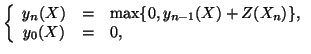
The non-parametric CUSUM algorithm works as follows. First we define
sequence
![]() :
:
| (1) |
One might suggest that we apply the CUSUM algorithm directly on random
sequence
![]() or
or
![]() to detect fast scanning
IM worms spreading by file transfers or URL-embedded chat messages. A
basic assumption of the CUSUM algorithm, however, is that the process
before the change point should be stationary. It is easy to see that
both random sequences
to detect fast scanning
IM worms spreading by file transfers or URL-embedded chat messages. A
basic assumption of the CUSUM algorithm, however, is that the process
before the change point should be stationary. It is easy to see that
both random sequences
![]() are
are
![]() vary with
the number of online users, which typically changes over the time in a
day. For instance, measurements of IM traffic in a large corporate
network reveal that the peak times of user login and user logout are
around 9AM and 5PM, respectively, which are strongly correlated with
employees' working hours [23]. If we attempt to
detect a fast scanning IM worm quickly by selecting a measurement
window
vary with
the number of online users, which typically changes over the time in a
day. For instance, measurements of IM traffic in a large corporate
network reveal that the peak times of user login and user logout are
around 9AM and 5PM, respectively, which are strongly correlated with
employees' working hours [23]. If we attempt to
detect a fast scanning IM worm quickly by selecting a measurement
window
![]() much smaller than a day, applying the CUSUM
algorithm directly on random sequence
much smaller than a day, applying the CUSUM
algorithm directly on random sequence
![]() or
or
![]() may lead to high false alarm rates.
may lead to high false alarm rates.
To circumvent this problem, we measure another random process
![]() , in which
, in which ![]() is the number of online IM users within the
is the number of online IM users within the
![]() -th measurement window
-th measurement window
![]() . Instead of detecting
abrupt changes on
. Instead of detecting
abrupt changes on
![]() or
or
![]() directly, we
normalize them by
directly, we
normalize them by ![]() first before applying the CUSUM
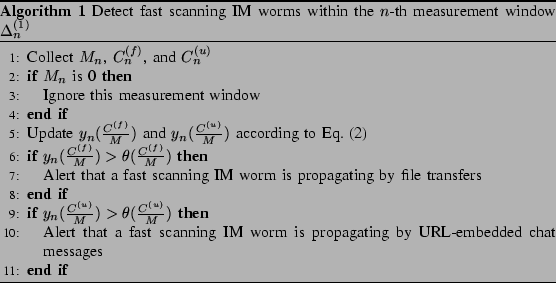
algorithm. Algorithm 1 provides a brief
overview of our solution to detecting fast scanning IM worms:
first before applying the CUSUM
algorithm. Algorithm 1 provides a brief
overview of our solution to detecting fast scanning IM worms:
When implementing Algorithm 1, if there
are no online IM users (i.e., ![]() ), we ignore this measurement
window, which means that the next measurement window is still the
), we ignore this measurement
window, which means that the next measurement window is still the
![]() -th measurement window.
-th measurement window.
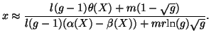
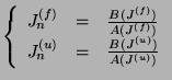
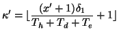
Parameter configuration. We set the model parameters in a
similar way as in [21]. First,
![]() and
and
![]() can be
estimated from training data. Define:
can be
estimated from training data. Define:
| (3) | |||
 |
(4) |
| (5) |
| (6) |
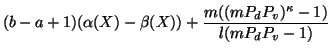
Algorithm analysis. We now analyze how effective the CUSUM
algorithm is in detecting fast scanning IM worms. We assume that a
machine attempts to spread the worm onto its online IM buddies
immediately after it gets infected. For simplicity, we also assume
that at the initial propagation stage, the number of buddies that have
already been infected can be ignored. Let ![]() be the average number of
online users and
be the average number of
online users and ![]() be the average number of online buddies of each
online user in the IM network when the IM worm is spreading. When an
infected machine attempts to spread the worm onto
be the average number of online buddies of each
online user in the IM network when the IM worm is spreading. When an
infected machine attempts to spread the worm onto ![]() online buddies,
online buddies,
![]() of them actually download the worm code. We assume that
the worm downloading time is
of them actually download the worm code. We assume that
the worm downloading time is ![]() . Hence, if an
infected machine initiates a successful infection attempt to an online
buddy at time
. Hence, if an
infected machine initiates a successful infection attempt to an online
buddy at time ![]() , the victim machine is infected at time
, the victim machine is infected at time
![]() . Among the
. Among the ![]() online buddies, an infected machine can
only infect
online buddies, an infected machine can
only infect ![]() of them successfully. Let
of them successfully. Let ![]() be the number
of worm generations before the worm is detected by the CUSUM
algorithm. The number of infected machines in the
be the number
of worm generations before the worm is detected by the CUSUM
algorithm. The number of infected machines in the ![]() -th worm
generation, where
-th worm
generation, where
![]() , is
, is
![]() . Suppose
that the IM worm starts to spread at the beginning of measurement
window
. Suppose
that the IM worm starts to spread at the beginning of measurement
window
![]() and the IM worm is detected at the end of
measurement window
and the IM worm is detected at the end of
measurement window
![]() . We then have:
. We then have:
| (8) |
 |
|||
 |
 |
(10) |
From Eq. (11), we observe that if ![]() is
high, or
is
high, or ![]() is chosen much larger than
is chosen much larger than ![]() , it takes a
longer time to detect the fast scanning IM worm, which is consistent
with our intuition.
, it takes a
longer time to detect the fast scanning IM worm, which is consistent
with our intuition.
Implementation. If Algorithm 1 is implemented by the IM servers, it needs to know the online status of each IM user. Such information is already available because the IM servers need to notify an IM user of each buddy's presence status when she just logs into the IM system. If Algorithm 1 is implemented at the enterprise gateway, there are two ways of keeping the online status of each internal IM user. One is to intercept every IM command that carries the presence information of an IM user. The second approach is to monitor the persistent TCP connections between the IM user and some IM servers, such as the BOS server in the AIM system and the notification server in the MSN system [23]: if such TCP connections are still alive, the corresponding IM user is online.
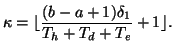
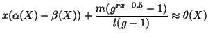
Security by obscurity is never a good practice. If an adversary knows
that Algorithm 1 has been deployed to
detect IM worms, can he design an intelligent IM worm that spreads
without being caught? We demonstrate its possibility in the following
discussion. Note that the CUSUM algorithm triggers an alarm only when
the cumulative sum reaches threshold ![]() ; this allows an IM
worm to ramp up its infection coverage using the fast scanning
strategy to a certain point without being detected. After that, the
difference between
; this allows an IM
worm to ramp up its infection coverage using the fast scanning
strategy to a certain point without being detected. After that, the
difference between ![]() and
and ![]() allows the IM worm to
spread at a constant speed without increasing
allows the IM worm to
spread at a constant speed without increasing ![]() . Following the
scenario analyzed in Section III, an
adversary estimates
. Following the
scenario analyzed in Section III, an
adversary estimates ![]() according to Eq. (11) and
predicts that a fast scanning IM is detected after
according to Eq. (11) and
predicts that a fast scanning IM is detected after ![]() measurement
windows. To avoid detection, the IM worm is designed to stop
propagating in a fast scanning mode after
measurement
windows. To avoid detection, the IM worm is designed to stop
propagating in a fast scanning mode after ![]() generations,
where:
generations,
where:
 |
(12) |
Since ![]() -th measurement window, the worm spreads in a
self-restraining manner. If the number of file transfer requests or
URL-embedded chat messages per measurement window generated by the
worm does not exceed
-th measurement window, the worm spreads in a
self-restraining manner. If the number of file transfer requests or
URL-embedded chat messages per measurement window generated by the
worm does not exceed
![]() , it is highly likely
that the worm propagates without triggering an alarm. We now show how
an intelligent IM worm can achieve this using a token-based
approach. Note that the number of infected machines in the
, it is highly likely
that the worm propagates without triggering an alarm. We now show how
an intelligent IM worm can achieve this using a token-based
approach. Note that the number of infected machines in the
![]() -th generation is
-th generation is
![]() , where we recall
, where we recall
![]() . Let
. Let ![]() be
be
![]() . After a
. After a
![]() -th worm instance is created,
-th worm instance is created,
![]() tokens are generated for
it.
tokens are generated for
it.
The color of a token can be green or red. Initially, we
set the colors of all tokens to green. The protocol works as follows:
(1) If the color of a token changes to green, the holding worm
instance randomly chooses a new victim that it has never tried to
infect from the online IM buddy list and then attempts to infect
it. If the holding worm instance cannot find an online buddy contact
that has never been tried, it passes the green token to a random
online buddy that it knows has already been infected, or to the
machine from which it gets infected; otherwise, it changes the color of the
token to red, inscribes the current time onto the token, and
schedules an activation timer which fires after ![]() time
units since the timestamp on the token. (2) When an activation
timer fires, the associated token changes to green and the holding
worm instance proceeds as in (1). (3) If a worm instance
successfully infects a new machine, it cancels any of its red tokens,
if it has such one, and passes it to the new machine without altering
its inscribed timestamp. (4) When a worm instance receives a red
token with time stamp
time
units since the timestamp on the token. (2) When an activation
timer fires, the associated token changes to green and the holding
worm instance proceeds as in (1). (3) If a worm instance
successfully infects a new machine, it cancels any of its red tokens,
if it has such one, and passes it to the new machine without altering
its inscribed timestamp. (4) When a worm instance receives a red
token with time stamp ![]() , it schedules an activation timer after
time
, it schedules an activation timer after
time
![]() , where
, where ![]() is the current time. (5) When
a worm instance receives a green token, it proceeds in the same way as
in (1). We can easily establish the following property of the
token-based protocol (proof omitted due to space limitation):
is the current time. (5) When
a worm instance receives a green token, it proceeds in the same way as
in (1). We can easily establish the following property of the
token-based protocol (proof omitted due to space limitation):
Algorithm description. We call intelligent IM worms that use rate limiting methods such as the token-based protocol self-restraining IM worms. To detect such type of IM worms, monitoring surges of file transfer requests or URL-embedded chat messages in the IM system is not sufficient. Instead, we measure likelihoods of file transfers or URL-embedded chat messages between IM clients and use them to decide whether a self-restraining IM worm is spreading. This idea is based on the measurements on IM messages in a large corporate network: on average, an AIM user chats with only 1.9 buddies, about 7% on her buddy list, and an MSN user chats with 5.5 buddies, 25% on her buddy list, in a month [23]. Such an observation suggests that an IM user tends to chat more often with a small set of her online buddies, which reflects her online social intimacy. However, self-restraining IM worms as described do not have that knowledge about social relationships between IM users. Hence, when an IM worm instance chooses a victim from the online buddy list, it randomly picks one from those that have not been attempted before. As such randomness may not reflect real-world online social intimacy, it offers a weakness for their detection.
Similar to Algorithm 1, we discretize
time into measurement windows of equal length ![]() , denoted by
, denoted by
![]() .
. ![]() is not
necessarily equal to
is not
necessarily equal to ![]() . Let
. Let ![]() and
and ![]() denote the set of IM user pairs
denote the set of IM user pairs
![]() , where IM user
, where IM user
![]() sends at least one file transfer request and at least one
URL-embedded chat message to IM user
sends at least one file transfer request and at least one
URL-embedded chat message to IM user ![]() within measurement window
within measurement window
![]() , respectively. We also use
, respectively. We also use ![]() to denote the
metric that reflects how close IM user
to denote the
metric that reflects how close IM user ![]() is to IM user
is to IM user ![]() in the IM
world. Essentially,
in the IM
world. Essentially, ![]() is the probability that IM user
is the probability that IM user ![]() sends a chat message or a file transfer request to
sends a chat message or a file transfer request to ![]() in the
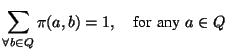
history. Let
in the
history. Let ![]() be the whole set of IM users. We have:
be the whole set of IM users. We have:
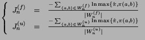
We define sequences
![]() and
and
![]() as follows:
as follows:
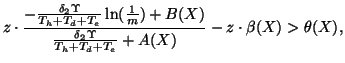
We then monitor abrupt change of
![]() and
and
![]() to
detect self-restraining IM worms:
to
detect self-restraining IM worms:
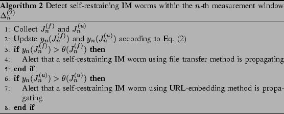
Parameters in Algorithm 2 are specified in a similar manner as in Algorithm 1. For brevity, we do not replicate it here.
Algorithm analysis. We consider the self-restraining IM worm
that uses the token-based scheme to control its propagation speed. The
total number of tokens is ![]() . We assume that at the initial
stage of worm propagation, each worm instance has received at most one
token. Also
let the number of online buddies per user be
. We assume that at the initial
stage of worm propagation, each worm instance has received at most one
token. Also
let the number of online buddies per user be ![]() . To ease analysis, we
further assume that under normal conditions, the nominators and
denominators in Eq. (15) are constant. That is,
. To ease analysis, we
further assume that under normal conditions, the nominators and
denominators in Eq. (15) are constant. That is,
 |
(17) |
From Eq. (18), it is clear that a too large
![]() or
or ![]() extends the detection period. But in
reality,
extends the detection period. But in
reality, ![]() and
and ![]() change over time. Hence, making
change over time. Hence, making ![]() or
or ![]() too small can introduce high false alarm rates.
too small can introduce high false alarm rates.
Implementation. One implementation issue with the
aforementioned algorithm is the complexity of collecting ![]() and
and ![]() . The algorithm requires knowledge of buddy
relationships in the IM system. If the algorithm is implemented at the
IM servers, such knowledge is already available, as the IM servers
need it to notify an IM client of the presence statuses of her buddies
if they change. For instance, in the AIM system, when an IM user logs
in, the client software sends a list of her IM buddies in screen names
to the message server; these names will be monitored for login/logout
events. If the detection algorithm is implemented at the enterprise
gateway, we need to parse IM command messages to derive buddy
relationships. For instance, the detection algorithm designed for the
AIM system can capture the ``oncoming buddy'' commands at the
enterprise gateway that appear in the following three cases: first,
the AIM messenger server notifies each user of the statuses of her
buddies when she is logging into the system; second, whenever one of
the buddies comes online after a user logged in, she gets a
notification from the servers; third, the IM servers regularly use
these commands to update the buddy list of each user [13].
. The algorithm requires knowledge of buddy
relationships in the IM system. If the algorithm is implemented at the
IM servers, such knowledge is already available, as the IM servers
need it to notify an IM client of the presence statuses of her buddies
if they change. For instance, in the AIM system, when an IM user logs
in, the client software sends a list of her IM buddies in screen names
to the message server; these names will be monitored for login/logout
events. If the detection algorithm is implemented at the enterprise
gateway, we need to parse IM command messages to derive buddy
relationships. For instance, the detection algorithm designed for the
AIM system can capture the ``oncoming buddy'' commands at the
enterprise gateway that appear in the following three cases: first,
the AIM messenger server notifies each user of the statuses of her
buddies when she is logging into the system; second, whenever one of
the buddies comes online after a user logged in, she gets a
notification from the servers; third, the IM servers regularly use
these commands to update the buddy list of each user [13].
Algorithm 2 also requires knowledge of
![]() from each online IM user
from each online IM user ![]() to each of her buddies
to each of her buddies ![]() . As
text-based chat messages and file transfer requests go through IM
servers, we can calculate
. As
text-based chat messages and file transfer requests go through IM
servers, we can calculate ![]() by parsing IM chat messages or IM
command messages for setting up file transfers at the IM servers or
the enterprise gateway.
by parsing IM chat messages or IM
command messages for setting up file transfers at the IM servers or
the enterprise gateway.
We use a realistic MSN IM messaging dataset to evaluate the effectiveness of our algorithms in detecting IM worms. This dataset, collected from a large corporate network, records chat messages of internal IM users and their online durations within a year. Our experiments are based on part of this dataset that has ten weeks' records. This subset has 193 internal IM users; on average, each of them has 22 IM buddies. In total, 3851 external IM contacts appear on the buddy lists of these 193 internal IM users. Unfortunately, we cannot get the buddy lists of these external IM users. As observed in [12,17], IM networks tend to have power-law structures. We use the Power-Law Out-Degree Algorithm [15] to generate power-law graphs with 3581 nodes, whose average outdegree is 22. The power law exponent is set to be 1.7, based on measurement results from [12,17]. For simplicity, we let the buddy relationships in the external graph be symmetric. Furthermore, if an external user is on the buddy list of an internal user, she also has that internal user on her own buddy list.
In our experiments, we consider only IM worms that are based on file transfers. Due to some technical problems, we are not able to obtain sufficient data on normal file transfers between internal IM users or between internal IM users and external IM users as of writing. We thus use measurement results from [10]: on average an online IM user sends out 1.84 file transfer requests per 24 hours. Similarly, we assume that the average number of file transfer requires an IM user receives is also 1.84. For each file transfer request, the probability that it falls into a time interval is proportional to the number of online internal IM users; once the time interval is chosen, its exact appearance time at the enterprise gateway is uniformly distributed within that time interval.
Now we introduce how to generate the sender and receiver of a file
transfer request if it is issued by an internal IM user. For each of
the 193 internal IM users, we build a buddy relationship table, an
entry in which indicates the probability that a chat message is sent
from her to the corresponding contact on her buddy list within the
current week (i.e., not history based). These probabilities are
empirically measured from the IM dataset. Let
![]() denote the probability that a chat message goes from internal IM user
denote the probability that a chat message goes from internal IM user
![]() to another IM user
to another IM user ![]() . Also, we measure the probability that an
outbound chat message (i.e., it is generated from an internal IM user)
comes from a specific internal IM user
. Also, we measure the probability that an
outbound chat message (i.e., it is generated from an internal IM user)
comes from a specific internal IM user ![]() , denoted by
, denoted by
![]() . Then, when a file transfer request sent by an internal IM
user is generated within a time interval, we first collect the entire
set of IM user pairs
. Then, when a file transfer request sent by an internal IM
user is generated within a time interval, we first collect the entire
set of IM user pairs ![]() , where
, where ![]() is an internal IM user and
both IM users
is an internal IM user and
both IM users ![]() and
and ![]() are online during that time interval. Let
are online during that time interval. Let
![]() be this set. Then, IM user pair
be this set. Then, IM user pair ![]() is chosen with
probability
is chosen with
probability ![]() :
:
 |
(19) |
In the experiments, we assume that the delay in seconds from one IM
user to another obeys normal distribution
![]() in
seconds. The time that a recipient of a file transfer request spends
on deciding whether to accept the request is exponentially distributed
with mean 5 seconds. The downloading time is generated from normal
distribution
in
seconds. The time that a recipient of a file transfer request spends
on deciding whether to accept the request is exponentially distributed
with mean 5 seconds. The downloading time is generated from normal
distribution
![]() . We ignore the execution time of
downloaded malware in our experiments. We vary the acceptance ratio of
a file transfer request (i.e.,
. We ignore the execution time of
downloaded malware in our experiments. We vary the acceptance ratio of
a file transfer request (i.e., ![]() ) among 0.25, 0.5, 0.75, and
1.0. We also vary the vulnerable probability of a machine (i.e.,
) among 0.25, 0.5, 0.75, and
1.0. We also vary the vulnerable probability of a machine (i.e.,
![]() ) among 0.25, 0.5, 0.75, and 1.0.
) among 0.25, 0.5, 0.75, and 1.0.
For each simulation scenario, we randomly pick an IM node, either
internal or external, as the initial infection. The first infection
takes place at simulation time 42000 seconds. For each simulation
scenario, we run it 10 times with different random number generation
seeds. In our experiments, IM worm detection is performed at the
enterprise gateway.
|
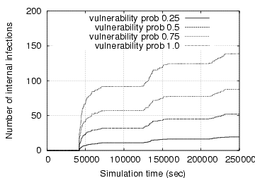
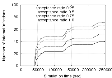
In Fig. 2, we present the growth
curves of internal infections (i.e., infected machines that are behind
the enterprise gateway) when the IM worm uses the fast scanning
spreading strategy. Obviously, when the acceptance ratio (i.e., ![]() )
is fixed, a higher percentage of vulnerable IM contacts leads to
faster IM worm spreading; similarly, when a fixed portion of IM
contacts is vulnerable, a higher acceptance ratio also accelerates IM
worm propagation. Both observations agree with our
intuition. Moreover, the maximum number of infected internal IM
contacts is bounded by the number of internal vulnerable
machines. This is confirmed in the right graph: the number of internal
infections is always less than 97 (recall that there are 193 internal
IM users in our dataset). However, this is not true when the
acceptance ratio is fixed at 50% and the vulnerable probability is
100%. It is because an IM user can receive multiple file transfer
requests from different buddies and accepting any one of them leads to
a new infection.
)
is fixed, a higher percentage of vulnerable IM contacts leads to
faster IM worm spreading; similarly, when a fixed portion of IM
contacts is vulnerable, a higher acceptance ratio also accelerates IM
worm propagation. Both observations agree with our
intuition. Moreover, the maximum number of infected internal IM
contacts is bounded by the number of internal vulnerable
machines. This is confirmed in the right graph: the number of internal
infections is always less than 97 (recall that there are 193 internal
IM users in our dataset). However, this is not true when the
acceptance ratio is fixed at 50% and the vulnerable probability is
100%. It is because an IM user can receive multiple file transfer
requests from different buddies and accepting any one of them leads to
a new infection.
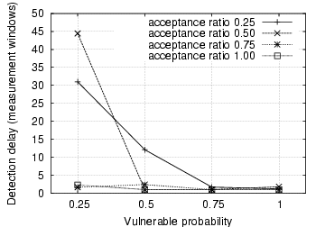
We now investigate how effective Algorithm
1 is in detecting these fast scanning IM
worms. We let the measurement window size be 300 seconds. The
threshold parameter is computed based on Eq. (7), in
which we let ![]() be 3 and
be 3 and ![]() be 3. Here, we choose a
relatively large
be 3. Here, we choose a
relatively large ![]() so that effects of white noise (e.g.,
bursts of normal file transfer requests) can be offset. We first test
the algorithm when there is no IM worm spreading. No false positives
have been observed. We then test 160 sample runs with 16 different
combinations of vulnerable probabilities and acceptance ratios. We
find that there are eight false negatives. A closer examination at the
eight false negatives reveals that in all of them either one (the
initial infection point) or two have been infected before simulation
time 250,000 seconds. Due to no widespread worm propagation, Algorithm
1 cannot detect it based on the number
of file transfer requests observed.
so that effects of white noise (e.g.,
bursts of normal file transfer requests) can be offset. We first test
the algorithm when there is no IM worm spreading. No false positives
have been observed. We then test 160 sample runs with 16 different
combinations of vulnerable probabilities and acceptance ratios. We
find that there are eight false negatives. A closer examination at the
eight false negatives reveals that in all of them either one (the
initial infection point) or two have been infected before simulation
time 250,000 seconds. Due to no widespread worm propagation, Algorithm
1 cannot detect it based on the number
of file transfer requests observed.
|
|
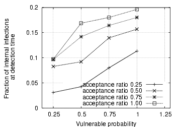
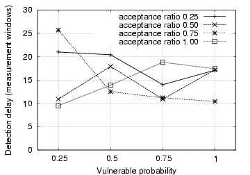
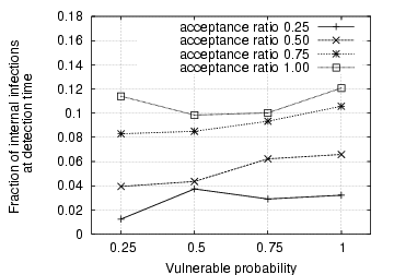
Fig. 3 depicts the detection delay in terms of measurement windows. For most of the scenarios, it takes between one and three measurement windows to detect the IM worm propagation. We, however, observe that when both the acceptance ratio and vulnerable probability are low, it takes a significant number of measurement windows to detect the IM worm. This is because in these cases the IM worm propagates very slowly and thus does not generate a large number of file transfer requests within a single measurement window. This is further confirmed in Fig. 4, which demonstrates the fraction of internal IM contacts that are infected among all internal vulnerable machines when the IM worm is detected. It is observed that for those cases with large detection delays, the fraction of internal infections is below 10%. On the other hand, when the vulnerable probability is 1.0, the fraction of internal infections reaches between 15% and 20% when the IM worm is detected, even though it takes only one measurement window. In these cases, we can accelerate IM worm detection by decreasing the measurement window size.
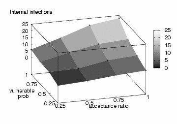
We now consider a self-restraining IM worm that limits its spreading speed to evade detection by Algorithm 1. This worm allows only three infection attempts (i.e., file transfer requests in our experiments) every 300 seconds. It uses the token-based protocol, as described in Section IV, to control its propagation speed. Fig. 5 depicts the number of internal infections at simulation time 250,000 seconds as a function of acceptance ratio and vulnerable probability. Compared against the fast scanning IM worm, the self-restraining IM worm propagates much more slowly. For instance, when the acceptance ratio is 50% and the vulnerable probability is 75%, the number of internal infections is only 9 after simulation time 250,000 seconds, as opposed to 88 internal infections with the fast scanning spreading strategy.
|
|
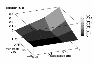
Fig. 6 presents the successful detection ratio of the self-restraining IM worm by Algorithm 1. Among 160 sample runs, Algorithm 1 can only catch 11 of them before simulation time 250,000 seconds. This leads to a poor average detection ratio of 7%. The result is not surprising because Algorithm 1 relies on the abrupt increase of file transfer requests for detection but the self-restraining IM worm generates only a limited number of file transfer requests per measurement window.
We now evaluate the effectiveness of Algorithm
2 in detecting self-restraining IM
worms. The measurement window ![]() used in this algorithm is
also set to be 300 seconds. We let the weighting factor
used in this algorithm is
also set to be 300 seconds. We let the weighting factor ![]() be
0.25 in Eq. (14) and parameter
be
0.25 in Eq. (14) and parameter ![]() be
be
![]() in Eq. (15). The
in Eq. (15). The ![]() parameter in
Eq. (14) is updated every week. Similar to the
experiments in Section V-A, we let both
parameter in
Eq. (14) is updated every week. Similar to the
experiments in Section V-A, we let both
![]() and
and ![]() be 3.
be 3.
The experimental results show that Algorithm 2 is able to detect the propagation of the self-restraining IM worm in all the 160 sample runs. Fig. 7 depicts the number of measurement windows that are needed to detect the IM worm under different combinations of acceptance ratios and vulnerable probabilities. The average detection delay is 16 measurement windows, which is equivalent to one hour and 20 minutes. Fig. 8 gives the fraction of internal infections among all internal vulnerable machines when the IM worm is detected. Obviously, only a small fraction of internal IM contacts has been infected before the IM worm is detected, suggesting that Algorithm 2 is effective in detecting self-restraining IM worms at their early stages.
IM malware has posed significant security threats to both residential and enterprise IM users. Mannan et al. presented a survey on secure public instant messaging in [9]. They later proposed to use limited throttling and CAPTCHA-based challenge-response schemes to defend against IM worms [10]; they also developed a cryptographic protocol to further enhance authentication and secure communications in public IM systems [11]. Smith analyzed a French language IM system and after observing the IM network is scale-free, he suggested that IM worms can be effectively mitigated by disabling the top few most connected IM accounts [17]. In [22], Williamson et al. demonstrated the effectiveness of a virus throttling algorithm against IM worm propagation. Xie et al. proposed a framework called HoneyIM that uses decoy IM accounts in normal users' buddy lists to detect IM propagation in enterprise-like networks [24]. Compared with previous solutions, our work focuses on a centralized approach that leverages statistical metrics collected from IM systems. As our solution does not require involvement of IM clients, it can be more easily deployed than those distributed detection schemes such as HoneyIM.
Applying change-point detection techniques to detect network attacks is not a new idea. Wang et al. applied the non-parametric CUSUM algorithm to detect TCP SYN flooding attacks [21]. The CUSUM algorithm has also been used to detect Internet worms in [2,3]. IM worms differ from traditional Internet worms such as Code Red II and Slammer because they propagate in social IM networks. In our work, we demonstrate that the change-point detection techniques are effective in catching IM worms with different spreading strategies.
In this paper, we have proposed to apply change-point detection techniques to detect both fast scanning and self-restraining IM worms. We monitor abrupt increase of file transfer requests or URL-embedded chat messages to detect fast scanning IM worms; we leverage social intimacy of IM users to detect stealthy IM worms that spread slowly. Experimental results show that the proposed solutions are effective in detecting both families of IM worms. We are currently developing algorithms for detecting another type of stealthy IM worms, which spread themselves between two online users only after they observe some ongoing conversations between them. In the future, we plan to evaluate the detection schemes proposed in this paper against more realistic IM datasets.
This document was generated using the LaTeX2HTML translator Version 2002 (1.62)
Copyright © 1993, 1994, 1995, 1996,
Nikos Drakos,
Computer Based Learning Unit, University of Leeds.
Copyright © 1997, 1998, 1999,
Ross Moore,
Mathematics Department, Macquarie University, Sydney.
The command line arguments were:
latex2html -split 0 -show_section_numbers -local_icons -no_navigation leet-im-worm.tex
The translation was initiated by Guanhua Yan on 2008-03-26